4. RNA-Seq expression example
Paul Harrison
2021-06-21
V4_airway.RmdLet’s look at the airway dataset as an example of a typical small-scale RNA-Seq experiment. In this experiment, four Airway Smooth Muscle (ASM) cell lines are treated with the asthma medication dexamethasone.
The function weitrix_calibrate_all will be used to assign precision weights to log Counts Per Million values.
library(weitrix)
library(ComplexHeatmap)
library(EnsDb.Hsapiens.v86)
library(edgeR)
library(limma)
library(reshape2)
library(tidyverse)
library(airway)

set.seed(1234)

# BiocParallel supports multiple backends.
# If the default hangs or errors, try others.
# The most reliable backed is to use serial processing
BiocParallel::register( BiocParallel::SerialParam() )
data("airway")
airway
## class: RangedSummarizedExperiment
## dim: 64102 8
## metadata(1): ''
## assays(1): counts
## rownames(64102): ENSG00000000003 ENSG00000000005 ... LRG_98 LRG_99
## rowData names(0):
## colnames(8): SRR1039508 SRR1039509 ... SRR1039520 SRR1039521
## colData names(9): SampleName cell ... Sample BioSampleInitial processing
Initial steps are the same as for a differential expression analysis.
counts <- assay(airway,"counts")

design <- model.matrix(~ dex + cell, data=colData(airway))

good <- filterByExpr(counts, design=design)
table(good)
## good
## FALSE TRUE
## 47242 16860
airway_dgelist <- DGEList(counts[good,]) %>% calcNormFactors()

airway_lcpm <- cpm(airway_dgelist, log=TRUE, prior.count=1)
log2 CPM values have been calculated, with an added “prior” count of (on average) 1 read, so that zeros aren’t sent to negative infinity.
Conversion to weitrix
airway_weitrix <- as_weitrix(airway_lcpm)

# Include row and column information
colData(airway_weitrix) <- colData(airway)
rowData(airway_weitrix) <-
    mcols(genes(EnsDb.Hsapiens.v86))[rownames(airway_weitrix),c("gene_name","gene_biotype")]

airway_weitrix
## class: SummarizedExperiment
## dim: 16860 8
## metadata(1): weitrix
## assays(2): x weights
## rownames(16860): ENSG00000000003 ENSG00000000419 ... ENSG00000273487
## ENSG00000273488
## rowData names(2): gene_name gene_biotype
## colnames(8): SRR1039508 SRR1039509 ... SRR1039520 SRR1039521
## colData names(9): SampleName cell ... Sample BioSampleCalibration
To calibrate, we need predicted expression levels so we can calculate residuals. The function weitrix_components can provide linear model fits to each gene. (We will see a more advanced use of this function later.)
fit <- weitrix_components(airway_weitrix, design=design)Currently the weitrix has weights uniformly equal to 1. Examining residuals, we see a variance trend relative to the linear model prediction.
Each dot in the plot below is a residual weighted by sqrt(weight). The x-axis is the linear model prediction. The y-axis is the weighted residual (all weights are currently 1). The red lines show the mean and the mean +/- one standard deviation.
weitrix_calplot(airway_weitrix, fit, covar=mu, guides=FALSE)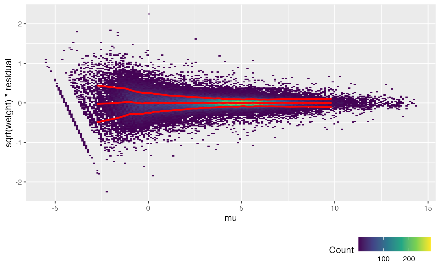
We will use the function weitrix_calibrate_all to set the weights by fitting a gamma GLM with log link function to the weighted squared residuals. 1 over the predictions from this GLM are used as weights. Here we fit a natural spline based on the linear model predictions from fit, which are referred to in the formula as mu. well_knotted_spline is a wrapper around splines::ns for natural splines with improved choice of knot locations.
airway_cal <- weitrix_calibrate_all(
    airway_weitrix,
    design = fit,
    trend_formula = ~well_knotted_spline(mu,5))
## mu range -5.552401 14.303375 knots -0.8637096 1.4763752 3.6914433 5.6106759 8.0243479
metadata(airway_cal)## $weitrix
## $weitrix$x_name
## [1] "x"
##
## $weitrix$weights_name
## [1] "weights"
##
## $weitrix$all_coef
## (Intercept) well_knotted_spline(mu, 5)1
## -0.4307917 -3.0128598
## well_knotted_spline(mu, 5)2 well_knotted_spline(mu, 5)3
## -4.0044737 -4.6128293
## well_knotted_spline(mu, 5)4 well_knotted_spline(mu, 5)5
## -3.3897229 -5.2701723
## well_knotted_spline(mu, 5)6
## -3.1086780
weitrix_calplot(airway_cal, fit, covar=mu)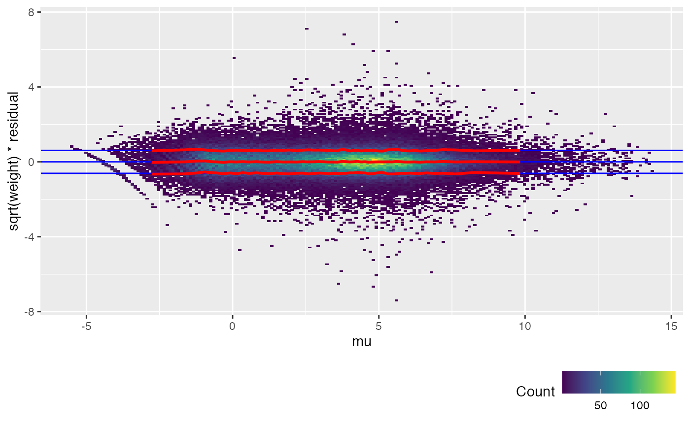
The trend lines (red) for the calibrated weitrix are now uniformly close to 1, 0, -1 (guide lines shown in blue). Weights can now be treated as inverse residual variance.
Another way to check this is to plot the unweighted residuals against 1/sqrt(weight), i.e. the residual standard deviation.
weitrix_calplot(airway_cal, fit, funnel=TRUE)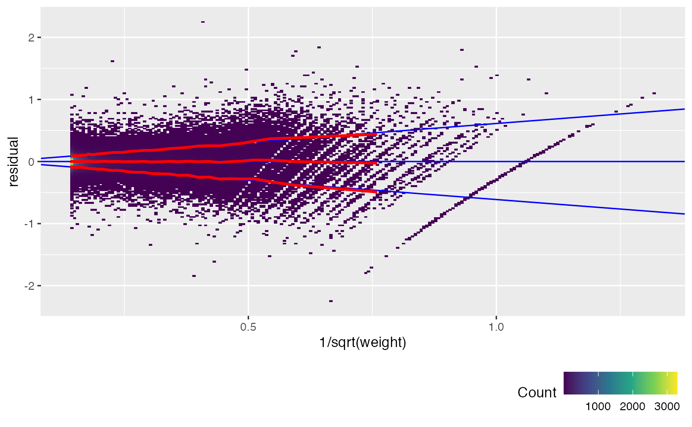
We can also check each sample individually.
weitrix_calplot(airway_cal, fit, covar=mu, cat=col)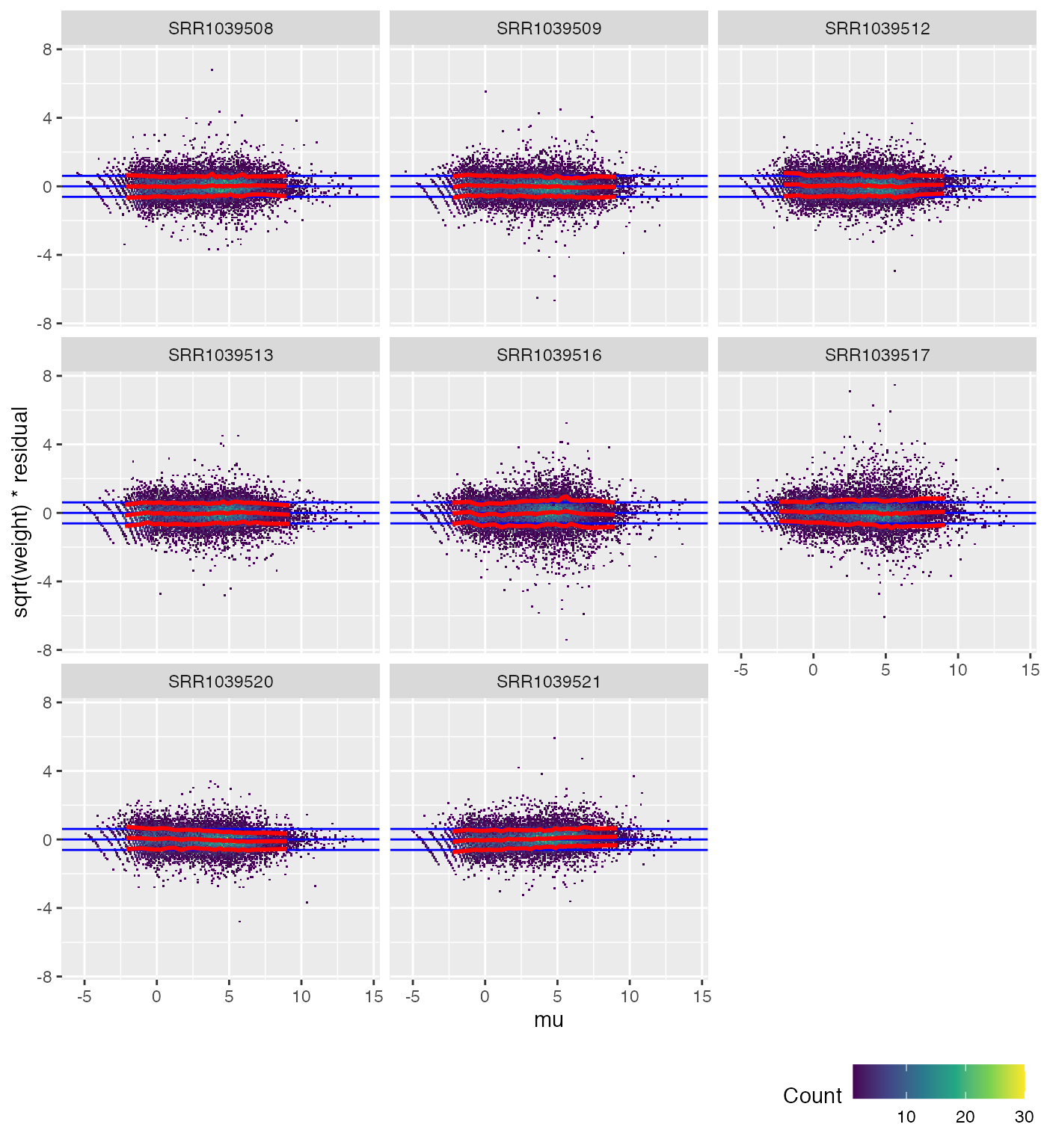
Advanced calibration
If there was an odd sample, we could use a more complex trend formula such as ~col*well_knotted_spline(mu,4):
airway_cal <- weitrix_calibrate_all(
    airway_weitrix,
    design = fit,
    trend_formula = ~col*well_knotted_spline(mu,4))
Similar to limma voom
While the precise details differ, what we have done is very similar to the voom function in limma.
weitrix_calplot can be used with voomed data as well.
airway_voomed <- voom(airway_dgelist, design, plot=TRUE)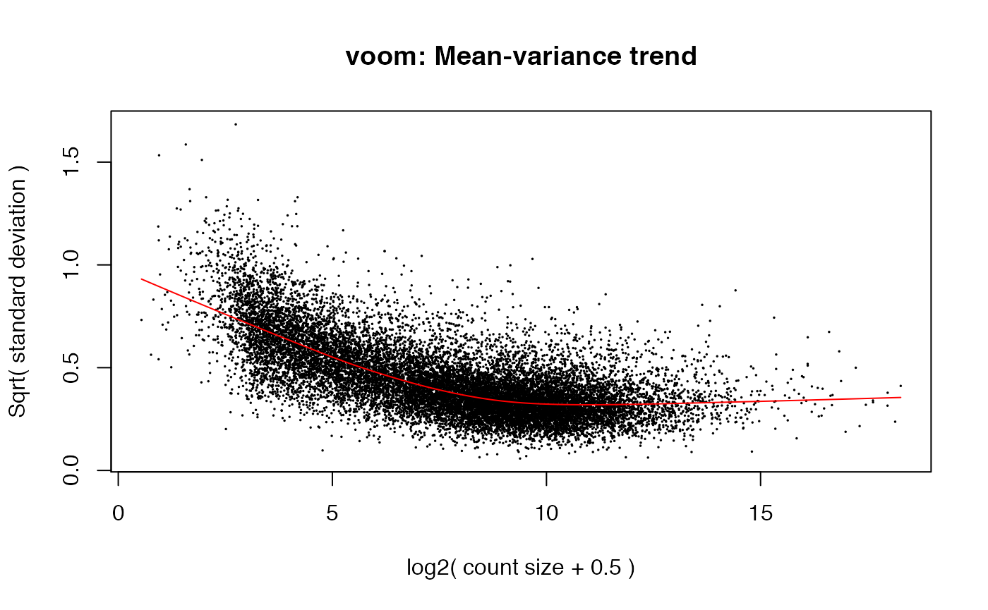
weitrix_calplot(airway_voomed, design, covar=mu)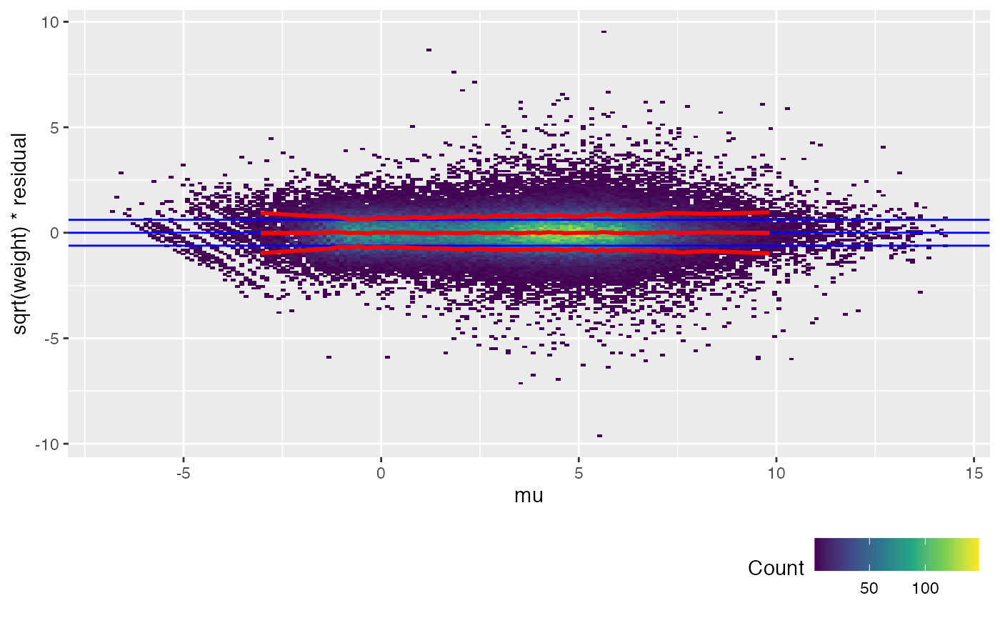
voom achieves a similar result to weitrix_calibrate_all (but note the input to voom is a DGEList of counts, not a matrix that is already log transformed). limma EList objects can be converted to weitrix objects with as_weitrix. Weitrix objects can be converted to limma EList objects with weitrix_elist.
Exploration
RNA-Seq expression is well trodden ground. The main contribution of the weitrix package here is to aid exploration by discovering components of variation, providing not just column scores but row loadings and respecting precision weights.
Find genes with excess variation
weitrix_sd_confects will find genes with excess variation in a calibrated weitrix.
confects <- weitrix_sd_confects(airway_cal)
confects
## $table
## confect effect row_mean typical_obs_err dispersion n_present df fdr_zero
## 1 2.620 3.121 6.631 0.2930 114.49 8 7 0
## 2 2.608 3.020 4.731 0.2495 147.49 8 7 0
## 3 2.368 2.785 3.850 0.2573 118.16 8 7 0
## 4 2.076 2.484 4.006 0.2557 95.41 8 7 0
## 5 2.009 2.271 8.249 0.1658 188.60 8 7 0
## 6 1.993 2.477 2.849 0.3102 64.79 8 7 0
## 7 1.905 2.208 4.396 0.1961 127.83 8 7 0
## 8 1.893 2.334 3.054 0.2875 66.93 8 7 0
## 9 1.892 2.145 6.065 0.1657 168.64 8 7 0
## 10 1.856 2.114 5.431 0.1702 155.23 8 7 0
## name gene_name gene_biotype
## 1 ENSG00000229807 XIST lincRNA
## 2 ENSG00000262902 MTCO1P40 processed_pseudogene
## 3 ENSG00000171819 ANGPTL7 protein_coding
## 4 ENSG00000243137 PSG4 protein_coding
## 5 ENSG00000123243 ITIH5 protein_coding
## 6 ENSG00000198732 SMOC1 protein_coding
## 7 ENSG00000162817 C1orf115 protein_coding
## 8 ENSG00000235750 KIAA0040 protein_coding
## 9 ENSG00000096060 FKBP5 protein_coding
## 10 ENSG00000204941 PSG5 protein_coding
## ...
## 6216 of 16860 non-zero excess standard deviation at FDR 0.05“effect” is root-mean-square variation in residuals relative to a fitted model in excess of what is expected from the calibrated weights. Here the model only has an intercept term, so the residuals represent variation from the weighted mean. “confect” scores are lower confidence bounds on the effect, adjusted for multiple testing using the topconfects method.
The default method assumes errors are normally distributed. If you have a large number of columns, this assumption can be relaxed. This is more appropriate for single cell data, which will typically have a large number of cells, and also not have normally distributed errors due to the sparse nature of the data. In single-cell experiments, this should be a good way to find marker genes.
confects2 <- weitrix_sd_confects(airway_cal, assume_normal=FALSE)
confects2
## $table
## confect effect row_mean typical_obs_err dispersion n_present df fdr_zero
## 1 2.4670 3.0204 4.73096 0.2495 147.49 8 7 2.569e-05
## 2 1.3842 2.3499 0.04261 0.5470 19.45 8 7 2.799e-03
## 3 0.7603 2.3745 1.94467 0.3821 39.62 8 7 1.468e-02
## 4 0.7603 2.1681 2.92166 0.2709 65.05 8 7 1.468e-02
## 5 0.7603 2.3265 2.71176 0.3267 51.70 8 7 1.468e-02
## 6 0.7141 2.1156 -0.41319 0.5607 15.24 8 7 1.468e-02
## 7 0.6611 2.3662 0.08127 0.5422 20.05 8 7 1.632e-02
## 8 0.6229 2.0476 2.12185 0.3153 43.17 8 7 1.632e-02
## 9 0.6189 2.2522 1.21883 0.4135 30.66 8 7 1.800e-02
## 10 0.3847 0.7536 8.80031 0.1657 21.68 8 7 1.468e-02
## name gene_name gene_biotype
## 1 ENSG00000262902 MTCO1P40 processed_pseudogene
## 2 ENSG00000221818 EBF2 protein_coding
## 3 ENSG00000144191 CNGA3 protein_coding
## 4 ENSG00000247627 MTND4P12 processed_pseudogene
## 5 ENSG00000178919 FOXE1 protein_coding
## 6 ENSG00000261239 ANKRD26P1 transcribed_unprocessed_pseudogene
## 7 ENSG00000226278 PSPHP1 unprocessed_pseudogene
## 8 ENSG00000248810 RP11-362F19.1 lincRNA
## 9 ENSG00000223722 RP11-467L13.5 processed_pseudogene
## 10 ENSG00000148175 STOM protein_coding
## ...
## 39 of 16860 non-zero excess standard deviation at FDR 0.05Top genes can then be examined to find a reason for their variation. For example, we see that XIST is highly expressed in a particular cell type.
interesting <- confects$table$index[1:20]

centered <- weitrix_x(airway_cal) - rowMeans(weitrix_x(airway_cal))
rownames(centered) <- rowData(airway_cal)$gene_name
Heatmap(
    centered[interesting,],
    name="log2 RPM\nvs row mean",
    cluster_columns=FALSE)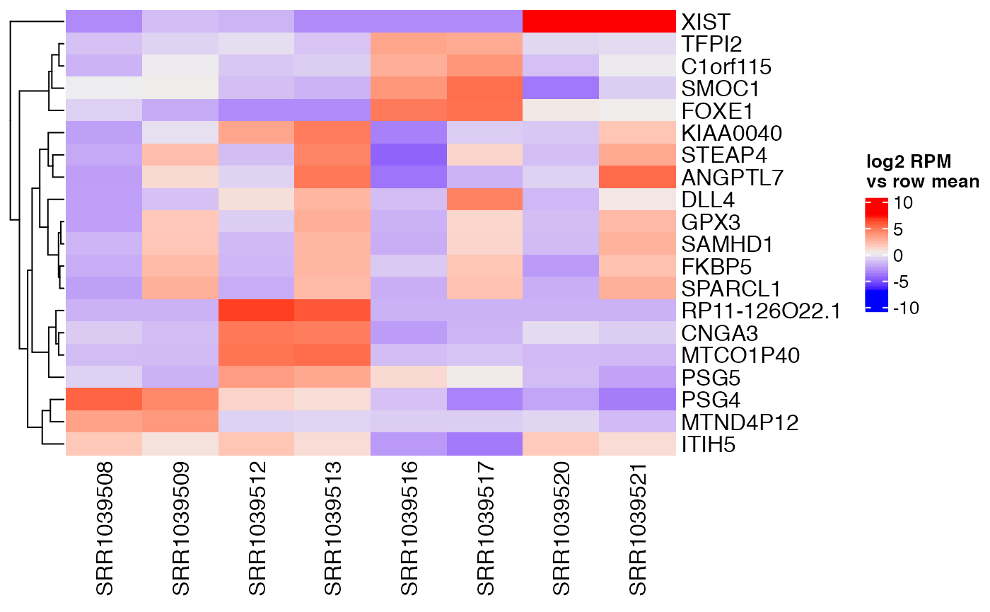
Find components of variation
The code below will find various numbers of components, from 1 to 6. In each case, the components discovered have varimax rotation applied to their gene loadings to aid interpretability. The result is a list of Components objects.
comp_seq <- weitrix_components_seq(airway_cal, p=6, n_restarts=1)
comp_seq
## [[1]]
## Components are: (Intercept), C1
## $row : 16860 x 2 matrix
## $col : 8 x 2 matrix
## $R2 : 0.4046082
##
## [[2]]
## Components are: (Intercept), C1, C2
## $row : 16860 x 3 matrix
## $col : 8 x 3 matrix
## $R2 : 0.6364208
##
## [[3]]
## Components are: (Intercept), C1, C2, C3
## $row : 16860 x 4 matrix
## $col : 8 x 4 matrix
## $R2 : 0.8055695
##
## [[4]]
## Components are: (Intercept), C1, C2, C3, C4
## $row : 16860 x 5 matrix
## $col : 8 x 5 matrix
## $R2 : 0.9096617
##
## [[5]]
## Components are: (Intercept), C1, C2, C3, C4, C5
## $row : 16860 x 6 matrix
## $col : 8 x 6 matrix
## $R2 : 0.9500206
##
## [[6]]
## Components are: (Intercept), C1, C2, C3, C4, C5, C6
## $row : 16860 x 7 matrix
## $col : 8 x 7 matrix
## $R2 : 0.9778973We can compare the proportion of variation explained to what would be explained in a completely random weitrix. Random normally distributed values are generated with variances equal to one over the weights.
rand_weitrix <- weitrix_randomize(airway_cal)
rand_comp <- weitrix_components(rand_weitrix, p=1, n_restarts=1)

components_seq_screeplot(comp_seq, rand_comp)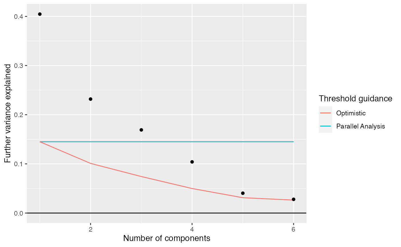
Examining components
Up to 4 components may be justified.
comp <- comp_seq[[4]]

comp$col[,-1] %>% melt(varnames=c("Run","component")) %>%
    left_join(as.data.frame(colData(airway)), by="Run") %>%
    ggplot(aes(y=cell, x=value, color=dex)) +
    geom_vline(xintercept=0) +
    geom_point(alpha=0.5, size=3) +
    facet_grid(~ component) +
    labs(title="Sample scores for each component", x="Sample score", y="Cell line", color="Treatment")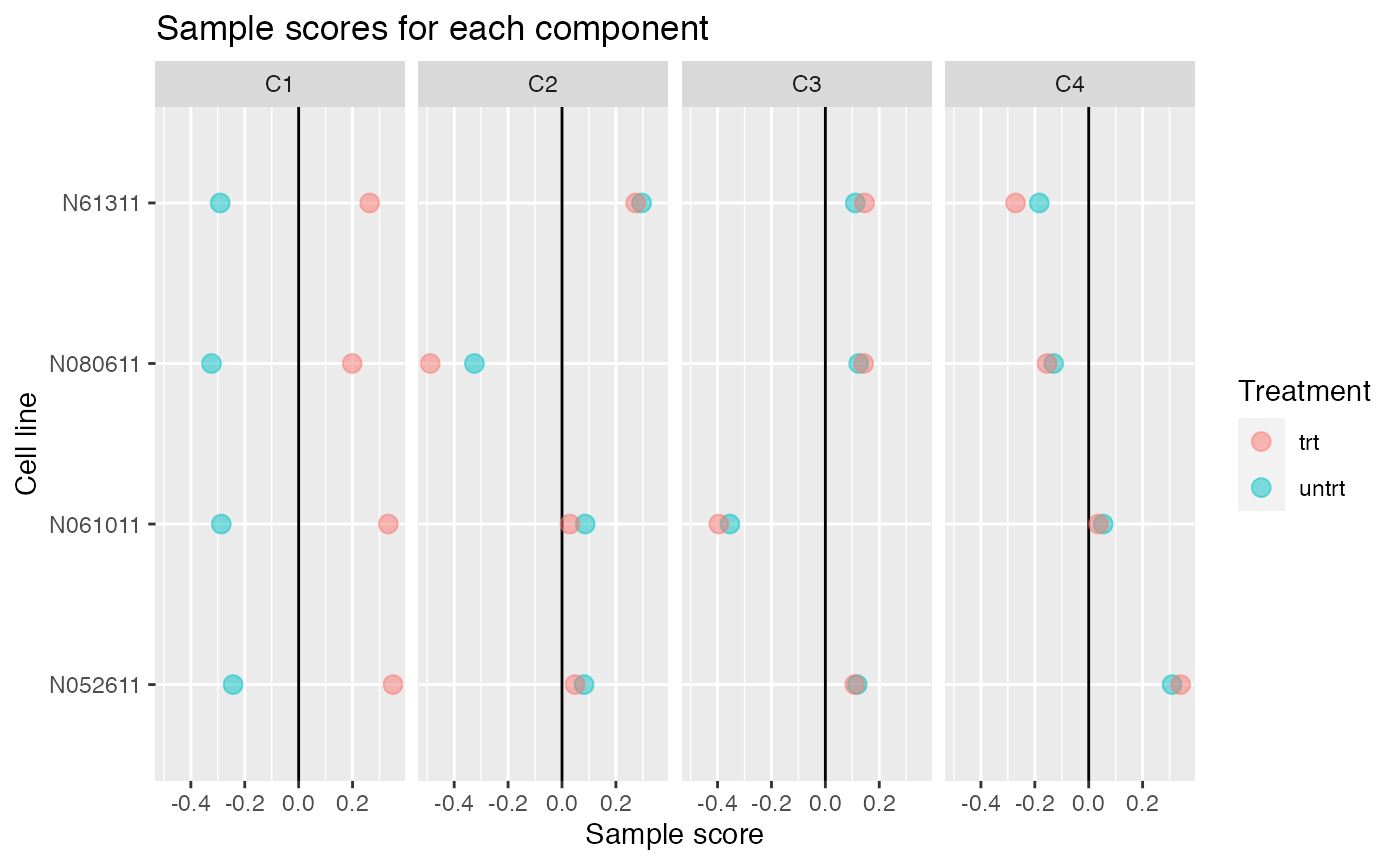
comp$row[,-1] %>% melt(varnames=c("name","component")) %>%
    ggplot(aes(x=comp$row[name,"(Intercept)"], y=value)) +
    geom_point(cex=0.5, alpha=0.5) +
    facet_wrap(~ component) +
    labs(title="Gene loadings for each component vs average log2 RPM", x="average log2 RPM", y="gene loading")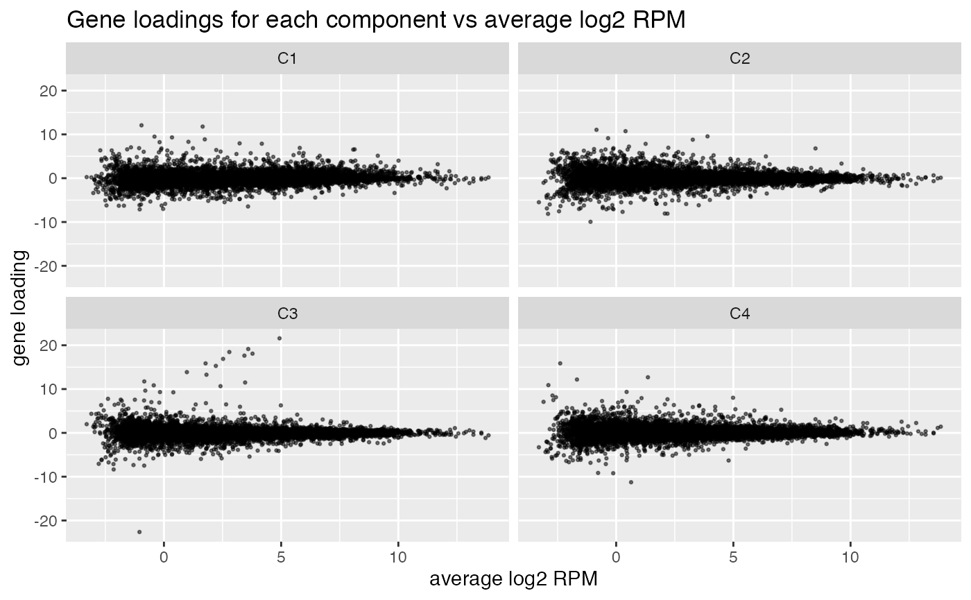
Without varimax rotation, components may be harder to interpret
If varimax rotation isn’t used, weitrix_components and weitrix_components_seq will produce a Principal Components Analysis, with components ordered from most to least variance explained.
Without varimax rotation the treatment effect is still mostly in the first component, but has also leaked a small amount into the other components.
comp_nonvarimax <- weitrix_components(airway_cal, p=4, use_varimax=FALSE)

comp_nonvarimax$col[,-1] %>% melt(varnames=c("Run","component")) %>%
    left_join(as.data.frame(colData(airway)), by="Run") %>%
    ggplot(aes(y=cell, x=value, color=dex)) +
    geom_vline(xintercept=0) +
    geom_point(alpha=0.5, size=3) +
    facet_grid(~ component) +
    labs(title="Sample scores for each component, no varimax rotation", x="Sample score", y="Cell line", color="Treatment")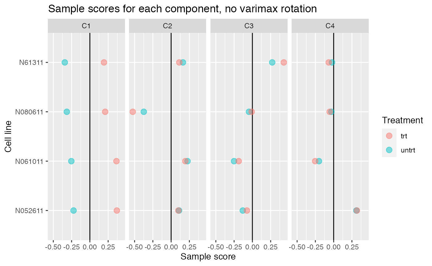
col can potentially be used as a design matrix
If you’re not sure of the experimental design, for example the exact timing of a time series or how evenly a drug treatment was applied, the extracted component might actually be more accurate.
Note that this ignores uncertainty about the col matrix itself.
This may be useful for hypothesis generation – finding some potentially interesting genes, while discounting noisy or lowly expressed genes – but don’t use it as proof of significance.
First by the topconfects method. This will find the largest confident effect sizes, while still correcting for multiple testing.
weitrix_confects(airway_cal, comp$col, "C1")## $table
## confect effect se df fdr_zero row_mean typical_obs_err
## 1 6.606 12.075 0.5919 9.195 2.653e-06 2.311 0.2012
## 2 6.463 11.783 0.6258 9.195 3.736e-06 4.755 0.2381
## 3 5.997 7.957 0.2423 9.195 3.073e-07 4.746 0.1522
## 4 5.956 9.320 0.4307 9.195 1.907e-06 3.850 0.2540
## 5 5.746 7.873 0.2799 9.195 4.763e-07 5.405 0.1935
## 6 5.510 6.586 0.1466 9.195 7.303e-08 7.758 0.1171
## 7 5.510 8.310 0.3843 9.195 1.907e-06 3.399 0.2057
## 8 5.236 8.871 0.5074 9.195 5.201e-06 4.021 0.2664
## 9 5.069 9.497 0.6276 9.195 1.135e-05 2.014 0.2745
## 10 -5.062 -6.453 0.1999 9.195 3.073e-07 4.648 0.1340
## name gene_name gene_biotype
## 1 ENSG00000179593 ALOX15B protein_coding
## 2 ENSG00000109906 ZBTB16 protein_coding
## 3 ENSG00000163884 KLF15 protein_coding
## 4 ENSG00000171819 ANGPTL7 protein_coding
## 5 ENSG00000152583 SPARCL1 protein_coding
## 6 ENSG00000101347 SAMHD1 protein_coding
## 7 ENSG00000168309 FAM107A protein_coding
## 8 ENSG00000127954 STEAP4 protein_coding
## 9 ENSG00000250978 RP11-357D18.1 processed_transcript
## 10 ENSG00000162692 VCAM1 protein_coding
## ...
## 5540 of 16860 non-zero contrast at FDR 0.05
## Prior df 6.2If you prefer limma and p-values:
airway_elist <- weitrix_elist(airway_cal)

fit <-
    lmFit(airway_elist, comp$col) %>%
    eBayes()

fit$df.prior
## [1] 6.19524
fit$s2.prior## [1] 0.5946888
topTable(fit, "C1")## gene_name gene_biotype logFC AveExpr t
## ENSG00000101347 SAMHD1 protein_coding 6.585680 8.135498 44.90834
## ENSG00000189221 MAOA protein_coding 5.730034 5.951528 34.04168
## ENSG00000178695 KCTD12 protein_coding -4.417195 6.452192 -31.72330
## ENSG00000139132 FGD4 protein_coding 3.809042 5.416374 31.54337
## ENSG00000179094 PER1 protein_coding 5.479478 4.423081 30.43529
## ENSG00000120129 DUSP1 protein_coding 5.120892 6.644985 29.38798
## ENSG00000162692 VCAM1 protein_coding -6.453409 3.576221 -32.29109
## ENSG00000124766 SOX4 protein_coding -4.273940 5.427907 -28.70344
## ENSG00000163884 KLF15 protein_coding 7.957297 3.249262 32.84342
## ENSG00000165995 CACNB2 protein_coding 5.717502 3.686989 29.63384
## P.Value adj.P.Val B
## ENSG00000101347 4.331667e-12 7.303191e-08 17.48757
## ENSG00000189221 5.456200e-11 3.073475e-07 15.61359
## ENSG00000178695 1.038475e-10 3.073475e-07 15.14447
## ENSG00000139132 1.093763e-10 3.073475e-07 15.08271
## ENSG00000179094 1.515295e-10 3.649695e-07 14.56555
## ENSG00000120129 2.084677e-10 3.905294e-07 14.51588
## ENSG00000162692 8.833396e-11 3.073475e-07 14.50721
## ENSG00000124766 2.583657e-10 4.356046e-07 14.30694
## ENSG00000163884 7.567087e-11 3.073475e-07 14.29881
## ENSG00000165995 1.932349e-10 3.905294e-07 14.13861
all_top <- topTable(fit, "C1", n=Inf, sort.by="none")
plotMD(fit, "C1", status=all_top$adj.P.Val <= 0.01)