3. PAT-Seq alternative polyadenylation example
Paul Harrison
2021-06-21
V3_shift.RmdAPA sites can be detected using the PAT-Seq protocol. This protocol produces 3’-end focussed reads. We examine GSE83162. This is a time-series experiment in which two strains of yeast are released into synchronized cell cycling and observed through two cycles. Yeast are treated with \(\alpha\)-factor, which causes them to stop dividing in antici… pation of a chance to mate. When the \(\alpha\)-factor is washed away, they resume cycling.
Shift score definition
Each gene has several APA sites, ordered from furthest upstrand to furthest downstrand. For each sample, we have a read count at each site.
For each gene:
We define the “shift” of a particular sample relative to all reads from all samples.
A “shift” score is first assigned to each site, being the proportion of all reads upstrand of the site minus the proportion of all reads downstrand of it (i.e. an average over all reads where upstrand reads are 1, downstrand reads are -1 and reads from the site itself are 0). The measurement for each sample is then an average over the site score for each read. The weight is the number of reads.
Shifts scores range from -1 to 1, and summarize whether upstrand (more negative) or downstrand (more positive) sites are being favoured. The weighted average score is zero.
The weights are the number of reads, however for a randomly chosen read we can estimate its variance based on the number of reads at each site and the site scores. (This estimate of variance includes any biological signal, so it’s not exactly a residual variance.) This is stored in the rowData() of the weitrix, and can be used to further calibrate weights. We prefer to defer this sort of calibration until after we’ve discoverd components of variation, as it tends to give high weight to genes with little APA. There are clearly some alternative choices to how weighting could be performed, and we hope the weitrix package gives you basic building blocks with which you can experiment!
Load files
library(tidyverse)    # ggplot2, dplyr, etc
library(patchwork)    # side-by-side ggplots
library(reshape2)     # melt()
library(weitrix)      # Matrices with precision weights

# Produce consistent results
set.seed(12345)

# BiocParallel supports multiple backends.
# If the default hangs or errors, try others.
# The most reliable backed is to use serial processing
BiocParallel::register( BiocParallel::SerialParam() )
peaks <- system.file("GSE83162", "peaks.csv.gz", package="weitrix") %>%
    read_csv()

counts <- system.file("GSE83162", "peak_count.csv.gz", package="weitrix") %>%
    read_csv() %>%
    column_to_rownames("name") %>%
    as.matrix()

genes <- system.file("GSE83162", "genes.csv.gz", package="weitrix") %>%
    read_csv() %>%
    column_to_rownames("name")

samples <- data.frame(sample=I(colnames(counts))) %>%
    extract(sample, c("strain","time"), c("(.+)-(.+)"), remove=FALSE) %>%
    mutate(
        strain=factor(strain,unique(strain)),
        time=factor(time,unique(time)))
rownames(samples) <- samples$sample

groups <- dplyr::select(peaks, group=gene_name, name=name)
# Note the order of this data frame is important
samples## sample strain time
## WT-tpre WT-tpre WT tpre
## WT-t0m WT-t0m WT t0m
## WT-t15m WT-t15m WT t15m
## WT-t30m WT-t30m WT t30m
## WT-t45m WT-t45m WT t45m
## WT-t60m WT-t60m WT t60m
## WT-t75m WT-t75m WT t75m
## WT-t90m WT-t90m WT t90m
## WT-t105m WT-t105m WT t105m
## WT-t120m WT-t120m WT t120m
## DeltaSet1-tpre DeltaSet1-tpre DeltaSet1 tpre
## DeltaSet1-t0m DeltaSet1-t0m DeltaSet1 t0m
## DeltaSet1-t15m DeltaSet1-t15m DeltaSet1 t15m
## DeltaSet1-t30m DeltaSet1-t30m DeltaSet1 t30m
## DeltaSet1-t45m DeltaSet1-t45m DeltaSet1 t45m
## DeltaSet1-t60m DeltaSet1-t60m DeltaSet1 t60m
## DeltaSet1-t75m DeltaSet1-t75m DeltaSet1 t75m
## DeltaSet1-t90m DeltaSet1-t90m DeltaSet1 t90m
## DeltaSet1-t105m DeltaSet1-t105m DeltaSet1 t105m
## DeltaSet1-t120m DeltaSet1-t120m DeltaSet1 t120m
head(groups, 10)## # A tibble: 10 x 2
## group name
## <chr> <chr>
## 1 YDR533C peak1653
## 2 YDR533C peak1652
## 3 YDR529C peak1648
## 4 YDR529C peak1647
## 5 snR84 peak1646
## 6 snR84 peak1645
## 7 snR84 peak1644
## 8 YDR524C-B peak1643
## 9 YDR524C-B peak1642
## 10 YDR500C peak1629
counts[1:10,1:5]## WT-tpre WT-t0m WT-t15m WT-t30m WT-t45m
## peak3910 58 24 46 54 41
## peak3911 25 9 24 28 18
## peak3912 7 9 10 13 18
## peak4139 30 4 7 12 13
## peak4140 8 1 1 8 2
## peak4141 55 7 13 19 20
## peak8533 37 35 42 64 47
## peak8534 38 50 44 53 36
## peak5235 16 4 2 7 4
## peak5236 14 5 2 5 4A “shift” weitrix is constructed based on a matrix of site-level counts, plus a data frame grouping sites into genes. The order of this data frame is important, earlier sites are considered upstrand of later sites.
wei <- counts_shift(counts, groups)## Calculating shifts in 1 blocks
colData(wei) <- cbind(colData(wei), samples)
rowData(wei)$symbol <- genes$symbol[match(rownames(wei), rownames(genes))]
Having obtained a weitrix, everthing discussed for the poly(A) tail length example is applicable here as well. We will only perform a brief exploratory analysis here.
Exploratory analysis
Components of variation
We can look for components of variation.
comp_seq <- weitrix_components_seq(wei, p=6, design=~0)
components_seq_screeplot(comp_seq)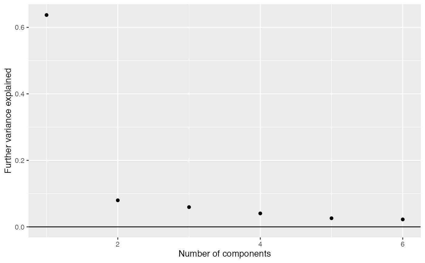
Pushing a point somewhat, we examine four components.
comp <- comp_seq[[4]]

matrix_long(comp$col, row_info=samples, varnames=c("sample","component")) %>%
    ggplot(aes(x=time, y=value, color=strain, group=strain)) +
    geom_hline(yintercept=0) +
    geom_line() +
    geom_point(alpha=0.75, size=3) +
    facet_grid(component ~ .) +
    labs(title="Sample scores for each component", y="Sample score", x="Time", color="Strain")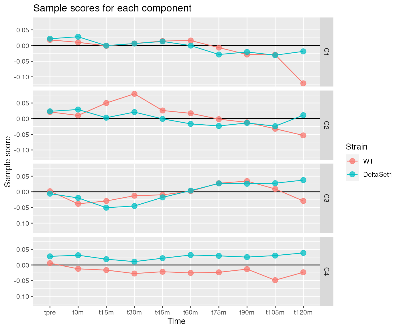
Calibration
Weights can be calibrated. Ideally the weights should be 1 over the residual variance. We will fit a gamma GLM with log link function to the squared residuals, and use the predictions from this to produce better weights. This model uses the per_read_var information present in the rowData, as well as applying a non-linear transformation to the existing weights.
cal <- weitrix_calibrate_all(
    wei,
    design = comp,
    trend_formula = ~log(per_read_var)+well_knotted_spline(log2(weight),3))
## log2(weight) range 0.00000 19.70383 knots 4.863982 7.206426 10.386132
metadata(cal)$weitrix$all_coef## (Intercept) log(per_read_var)
## 0.209536 1.185355
## well_knotted_spline(log2(weight), 3)1 well_knotted_spline(log2(weight), 3)2
## -4.692578 -5.234432
## well_knotted_spline(log2(weight), 3)3 well_knotted_spline(log2(weight), 3)4
## -9.261400 -6.398811A mean-variance trend is visible in the uncalibrated weighted residuals. Calibration has removed this, by making use of the information in per_read_var.
(weitrix_calplot(wei, comp, covar=mu) + labs(title="Before")) +
(weitrix_calplot(cal, comp, covar=mu) + labs(title="After"))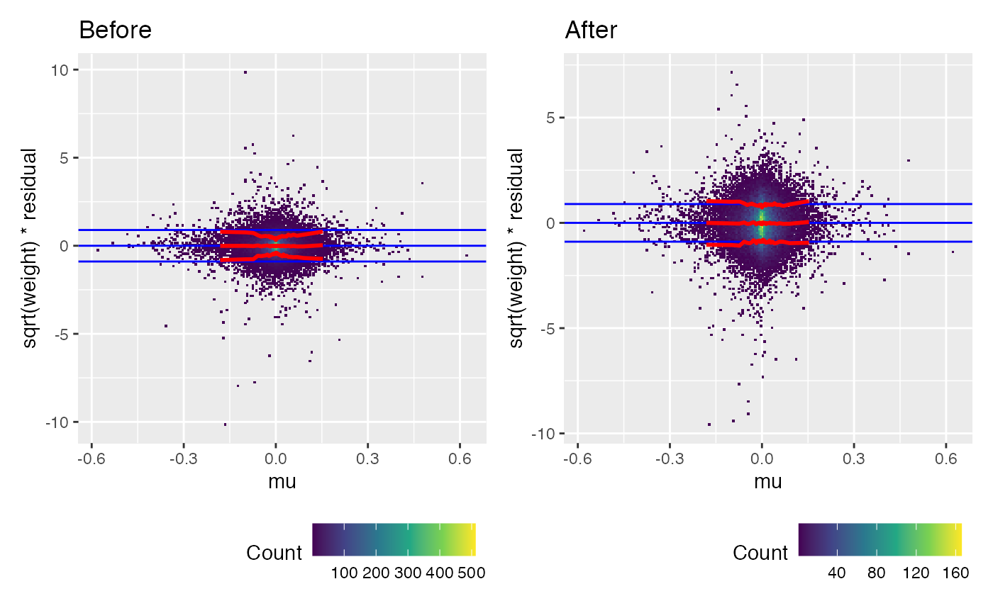
We can look at the calibration to per_read_var directly.
(weitrix_calplot(wei, comp, covar=per_read_var) + labs(title="Before")) +
(weitrix_calplot(cal, comp, covar=per_read_var) + labs(title="After"))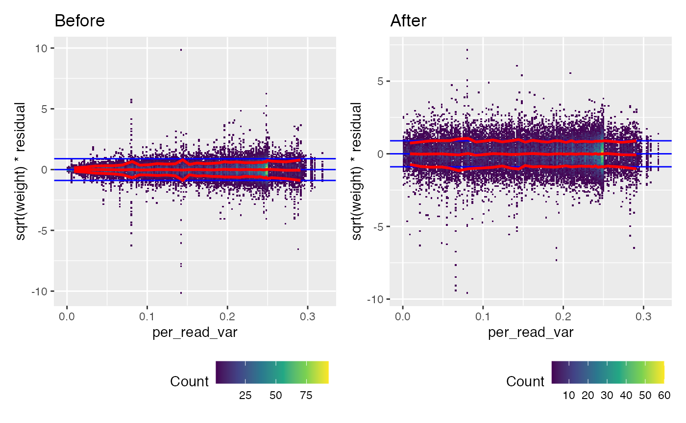
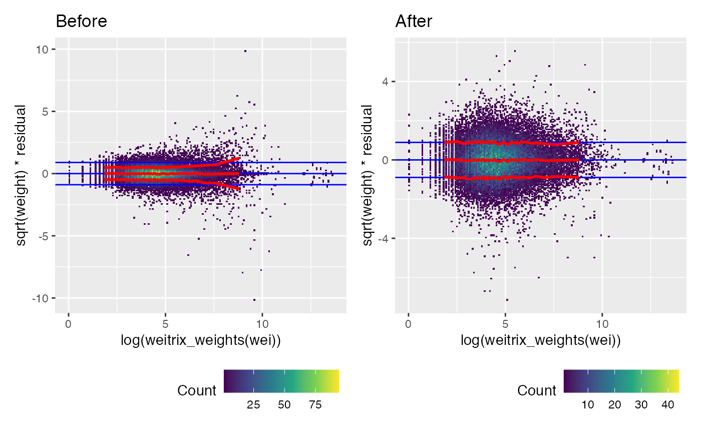
Weights were too large for large read counts. Calibration has applied a non-linear transformation to the weights that fixes this.
(weitrix_calplot(wei, comp, covar=log(weitrix_weights(wei))) + labs(title="Before")) +
(weitrix_calplot(cal, comp, covar=log(weitrix_weights(wei))) + labs(title="After"))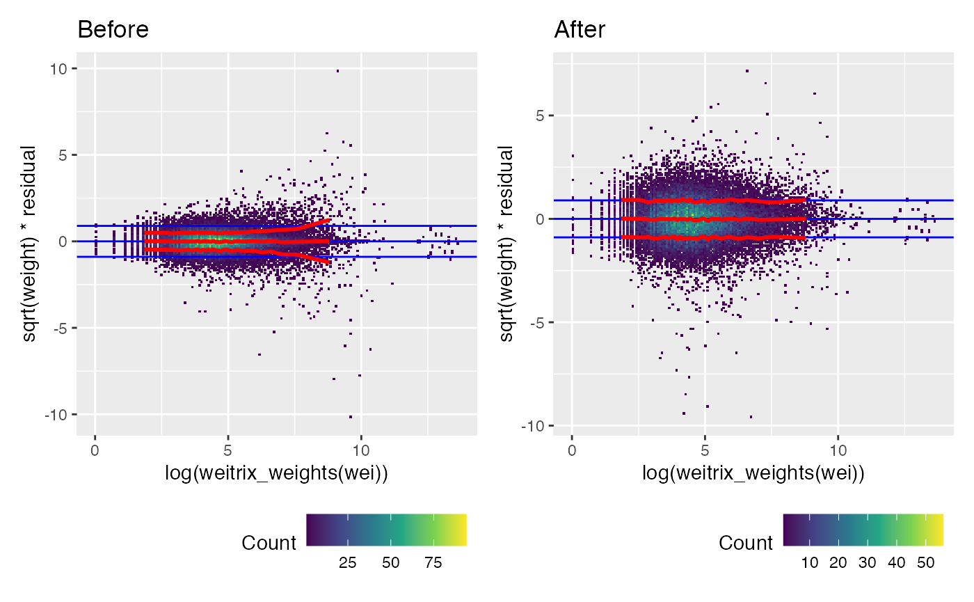
Another way of looking at this is with a “funnel” plot of 1/sqrt(weight) vs residuals. This should make a cone shape. Note how before calibration the pointy end of the cone is too wide.
(weitrix_calplot(wei, comp, funnel=TRUE, guides=FALSE) + labs(title="Before")) +
(weitrix_calplot(cal, comp, funnel=TRUE, guides=FALSE) + labs(title="After"))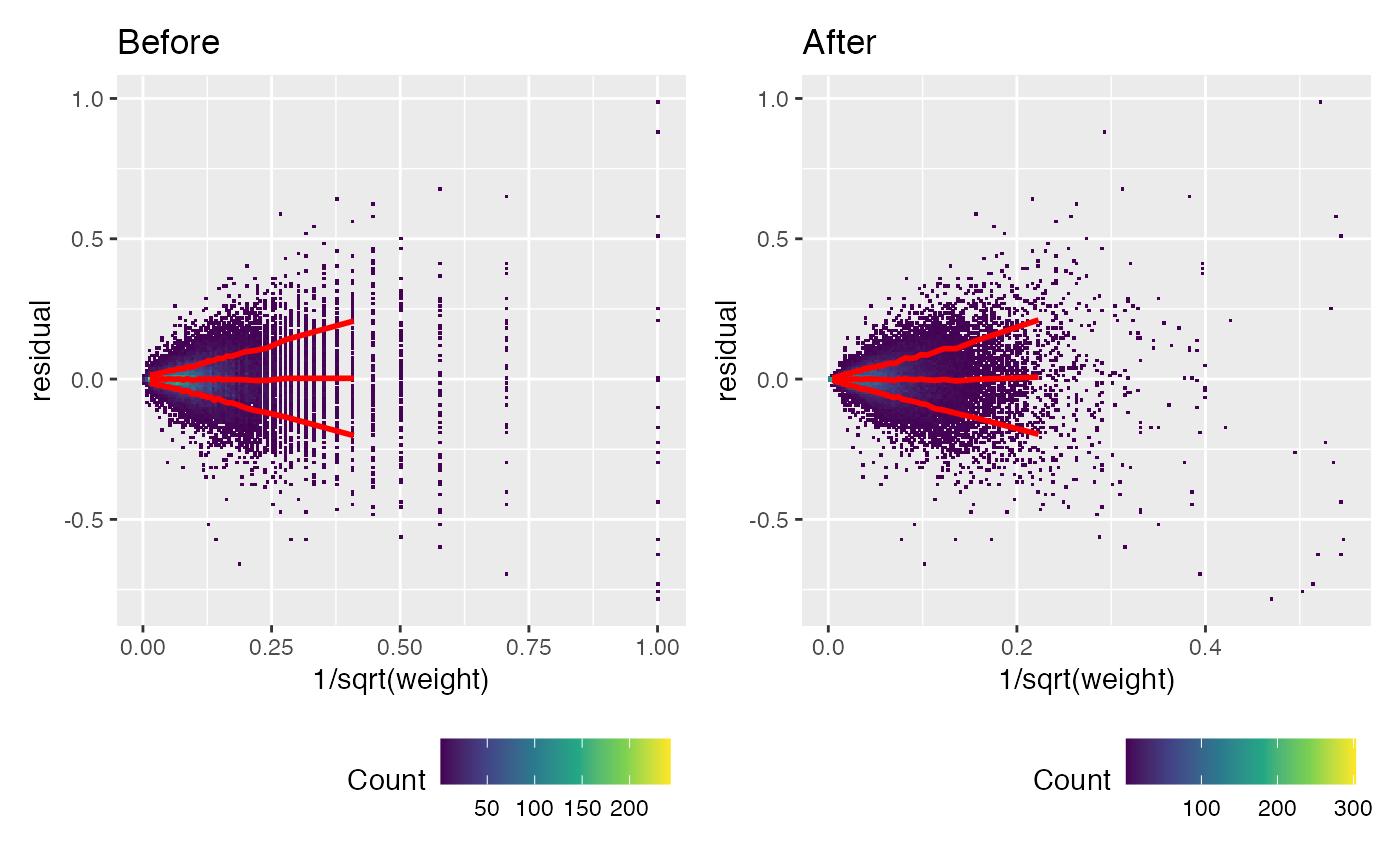
Using the calibrated weitrix with weitrix_confects
We will estimate confident loadings for the different components using weitrix_confects.
Treat these results with caution. Confindence bounds take into account uncertainty in the loadings but not in the scores! What follows is best regarded as exploratory rather than a final result.
Gene loadings for C1
weitrix_confects(cal, comp$col, "C1", fdr=0.05)## $table
## confect effect se df fdr_zero row_mean typical_obs_err name
## 1 2.576 4.084 0.3277 34.29 7.106e-12 -0.0045725 0.03724 YLR058C
## 2 2.258 3.278 0.2334 34.29 3.992e-13 0.0005282 0.02558 YPR080W
## 3 1.952 2.755 0.1898 34.29 2.000e-13 -0.0102218 0.02056 YKL096W-A
## 4 1.893 2.612 0.1741 34.29 1.117e-13 -0.0038158 0.01827 YBL072C
## 5 1.841 3.214 0.3390 34.29 6.749e-09 -0.0050486 0.03714 YBR127C
## 6 1.819 2.649 0.2082 34.29 4.559e-12 -0.0064119 0.02184 YML026C
## 7 1.511 3.844 0.5930 34.29 1.543e-05 -0.0035550 0.06222 YDR342C
## 8 1.439 2.344 0.2328 34.29 1.786e-09 -0.0127901 0.02361 YKL180W
## 9 1.408 1.978 0.1483 34.29 1.412e-12 -0.0062280 0.01556 YDR524C-B
## 10 1.363 2.305 0.2474 34.29 9.090e-09 -0.0077177 0.02540 YBR249C
## per_read_var total_reads symbol
## 1 0.18682 6958 SHM2
## 2 0.20630 72240 TEF1
## 3 0.08003 374176 CWP2
## 4 0.12048 47370 RPS8A
## 5 0.19376 21804 VMA2
## 6 0.11684 42444 RPS18B
## 7 0.16038 2866 HXT7
## 8 0.17678 57320 RPL17A
## 9 0.12464 164069 <NA>
## 10 0.16609 15246 ARO4
## ...
## 122 of 1805 non-zero contrast at FDR 0.05
## Prior df 18.3Gene loadings for C2
weitrix_confects(cal, comp$col, "C2", fdr=0.05)## $table
## confect effect se df fdr_zero row_mean typical_obs_err name
## 1 5.352 6.726 0.2984 34.29 3.493e-19 0.033448 0.02503 YLL024C
## 2 4.851 6.311 0.3344 34.29 6.577e-17 0.025712 0.02959 YLR333C
## 3 4.207 4.856 0.1535 34.29 1.065e-23 0.026578 0.01405 YLR110C
## 4 3.359 5.009 0.3997 34.29 8.439e-12 0.020404 0.03612 YKL081W
## 5 3.315 5.472 0.5323 34.29 1.344e-09 0.010999 0.04920 YBR135W
## 6 2.581 4.558 0.4955 34.29 1.441e-08 0.030207 0.04312 YDR363W-A
## 7 2.331 4.596 0.5756 34.29 2.644e-07 -0.001391 0.05256 YNL098C
## 8 2.331 3.767 0.3700 34.29 1.506e-09 0.008159 0.03437 YNL067W
## 9 2.331 5.570 0.8420 34.29 7.508e-06 0.008115 0.07561 YBR269C
## 10 2.313 4.006 0.4445 34.29 2.005e-08 0.014316 0.03827 YJL111W
## per_read_var total_reads symbol
## 1 0.1960 133748 SSA2
## 2 0.2382 46413 RPS25B
## 3 0.2070 712909 CCW12
## 4 0.2490 104942 TEF4
## 5 0.2461 3619 CKS1
## 6 0.1454 21193 SEM1
## 7 0.2405 7185 RAS2
## 8 0.2809 30030 RPL9B
## 9 0.2497 2289 SDH8
## 10 0.2001 14445 CCT7
## ...
## 165 of 1805 non-zero contrast at FDR 0.05
## Prior df 18.3Gene loadings for C3
weitrix_confects(cal, comp$col, "C3", fdr=0.05)## $table
## confect effect se df fdr_zero row_mean typical_obs_err name
## 1 1.304 2.684 0.3137 34.29 9.124e-07 0.0135791 0.03458 YBR149W
## 2 1.304 3.153 0.4234 34.29 1.048e-05 -0.0180649 0.04715 YDR077W
## 3 1.241 3.990 0.6581 34.29 2.499e-04 0.0018147 0.07298 YFR052C-A
## 4 1.241 4.219 0.7215 34.29 2.642e-04 0.0083707 0.07331 snR40
## 5 -1.195 -3.763 0.6385 34.29 2.584e-04 -0.0042835 0.07000 YMR194C-B
## 6 1.195 3.131 0.4853 34.29 1.305e-04 -0.0013908 0.05256 YNL098C
## 7 -0.605 -3.636 0.7707 34.29 3.720e-03 -0.0156241 0.08879 YKL163W
## 8 -0.605 -2.540 0.5005 34.29 1.875e-03 0.0004134 0.05319 YNL130C
## 9 0.605 3.627 0.7851 34.29 4.287e-03 -0.0063788 0.08470 YGR243W
## 10 -0.597 -1.686 0.2859 34.29 2.584e-04 -0.0085619 0.03087 YLR372W
## per_read_var total_reads symbol
## 1 0.19814 9498 ARA1
## 2 0.07946 66406 SED1
## 3 0.14798 4967 <NA>
## 4 0.26488 3100 <NA>
## 5 0.23748 2270 CMC4
## 6 0.24047 7185 RAS2
## 7 0.13916 808 PIR3
## 8 0.23029 4144 CPT1
## 9 0.23448 1172 MPC3
## 10 0.20219 20547 ELO3
## ...
## 112 of 1805 non-zero contrast at FDR 0.05
## Prior df 18.3Gene loadings for C4
weitrix_confects(cal, comp$col, "C4", fdr=0.05)## $table
## confect effect se df fdr_zero row_mean typical_obs_err name
## 1 3.912 6.544 0.5796 34.29 7.700e-10 0.019192 0.06693 RDN5-1
## 2 -3.912 -6.843 0.6713 34.29 3.891e-09 0.022990 0.07168 YIL015W
## 3 1.393 4.513 0.7380 34.29 1.335e-04 0.011478 0.08226 tK(CUU)M
## 4 1.283 4.387 0.7518 34.29 2.251e-04 -0.001030 0.08286 YLR286C
## 5 1.163 3.314 0.5310 34.29 1.044e-04 -0.006542 0.06112 tK(CUU)J
## 6 1.101 4.717 0.9153 34.29 7.379e-04 0.004439 0.09930 tP(UGG)O3
## 7 1.101 2.915 0.4610 34.29 1.044e-04 0.002452 0.05015 YJL054W
## 8 -1.098 -2.335 0.3188 34.29 7.473e-06 0.001259 0.03544 YLR027C
## 9 1.098 3.115 0.5245 34.29 2.001e-04 0.018252 0.05457 YCR009C
## 10 -0.973 -2.785 0.4758 34.29 2.251e-04 -0.001391 0.05256 YNL098C
## per_read_var total_reads symbol
## 1 0.2395 4029 <NA>
## 2 0.2090 4313 BAR1
## 3 0.2882 2843 <NA>
## 4 0.2424 1548 CTS1
## 5 0.0900 1200 <NA>
## 6 0.2500 892 <NA>
## 7 0.1756 1918 TIM54
## 8 0.2498 12186 AAT2
## 9 0.2292 5560 RVS161
## 10 0.2405 7185 RAS2
## ...
## 172 of 1805 non-zero contrast at FDR 0.05
## Prior df 18.3Genes with high variability
Instead of looking for genes following some particular pattern, we can look for genes that simply have surprisingly high variability with weitrix_sd_confects.
weitrix_sd_confects(cal, step=0.01)## $table
## confect effect row_mean typical_obs_err dispersion n_present df fdr_zero
## 1 0.18 0.2051 0.0204037 0.02667 60.129 20 19 0.000e+00
## 2 0.15 0.1793 0.0005282 0.02551 50.393 20 19 0.000e+00
## 3 0.15 0.1828 0.0257121 0.03040 37.156 20 19 0.000e+00
## 4 0.15 0.1976 0.0229903 0.05194 15.471 20 19 0.000e+00
## 5 0.15 0.1874 -0.0045725 0.03961 23.389 20 19 0.000e+00
## 6 0.14 0.1892 0.0191925 0.05425 13.165 20 19 0.000e+00
## 7 0.14 0.1700 -0.0050486 0.03110 30.885 20 19 0.000e+00
## 8 0.13 0.2445 0.0129646 0.12069 5.105 19 18 1.069e-10
## 9 0.13 0.1901 0.0081152 0.06682 9.095 20 19 0.000e+00
## 10 0.13 0.1488 0.0334475 0.02250 44.729 20 19 0.000e+00
## name per_read_var total_reads symbol
## 1 YKL081W 0.2490 104942 TEF4
## 2 YPR080W 0.2063 72240 TEF1
## 3 YLR333C 0.2382 46413 RPS25B
## 4 YIL015W 0.2090 4313 BAR1
## 5 YLR058C 0.1868 6958 SHM2
## 6 RDN5-1 0.2395 4029 <NA>
## 7 YBR127C 0.1938 21804 VMA2
## 8 tP(UGG)N1 0.2328 507 <NA>
## 9 YBR269C 0.2497 2289 SDH8
## 10 YLL024C 0.1960 133748 SSA2
## ...
## 470 of 1805 non-zero excess standard deviation at FDR 0.05Examine individual genes
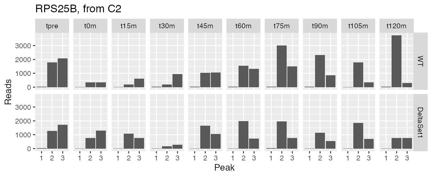
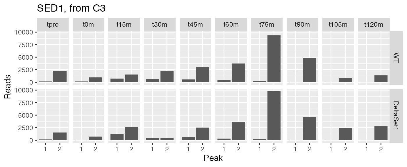
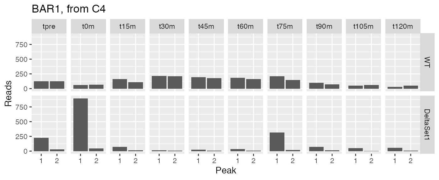
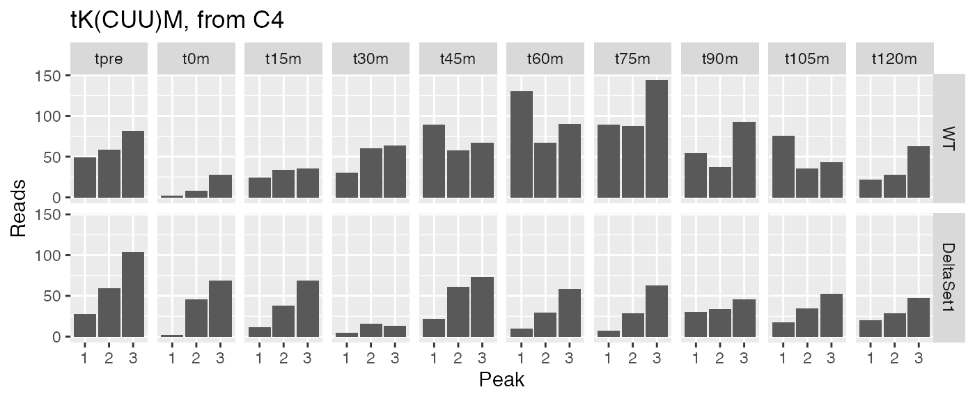
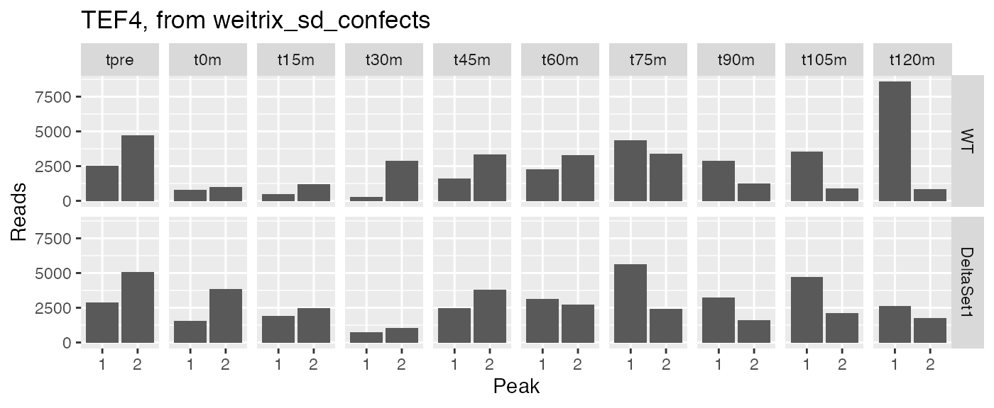
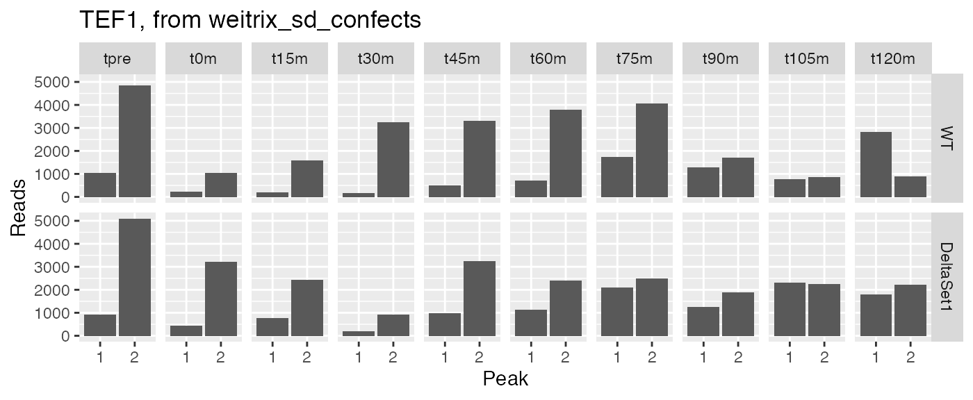
Let’s examine peak-level read counts for some genes we’ve identified.
examine <- function(gene_wanted, title) {
    peak_names <- filter(peaks, gene_name==gene_wanted)$name

    counts[peak_names,] %>% melt(value.name="reads", varnames=c("peak","sample")) %>%
        left_join(samples, by="sample") %>%
        ggplot(aes(x=factor(as.integer(peak)), y=reads)) +
        facet_grid(strain ~ time) + geom_col() +
        labs(x="Peak",y="Reads",title=title)
}

examine("YLR058C", "SHM2, from C1")
examine("YLR333C", "RPS25B, from C2")
examine("YDR077W", "SED1, from C3")
examine("YIL015W", "BAR1, from C4")
examine("tK(CUU)M", "tK(CUU)M, from C4")
examine("YKL081W", "TEF4, from weitrix_sd_confects")
examine("YPR080W", "TEF1, from weitrix_sd_confects")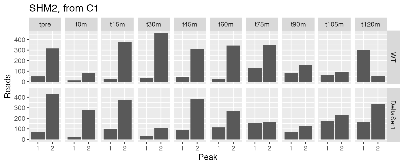
Alternative calibration method
For larger datasets, weitrix_calibrate_all may use a lot of memory. The weitrix packages also has an older version of calibration, weitrix_calibrate_trend. Rather than operating on weights individually, it applies a scaling to the weights of each row.
cal_trend <- weitrix_calibrate_trend(
    wei,
    design = comp,
    trend_formula = ~log(per_read_var)+well_knotted_spline(log(total_reads),3))
## log(total_reads) range 5.214936 16.049079 knots 6.749379 8.203755 10.367033A mean-variance trend is visible in the uncalibrated weighted residuals. Calibration removes this, by making use of the information in per_read_var.
(weitrix_calplot(wei, comp, covar=mu) + labs(title="Before")) +
(weitrix_calplot(cal_trend, comp, covar=mu) + labs(title="After"))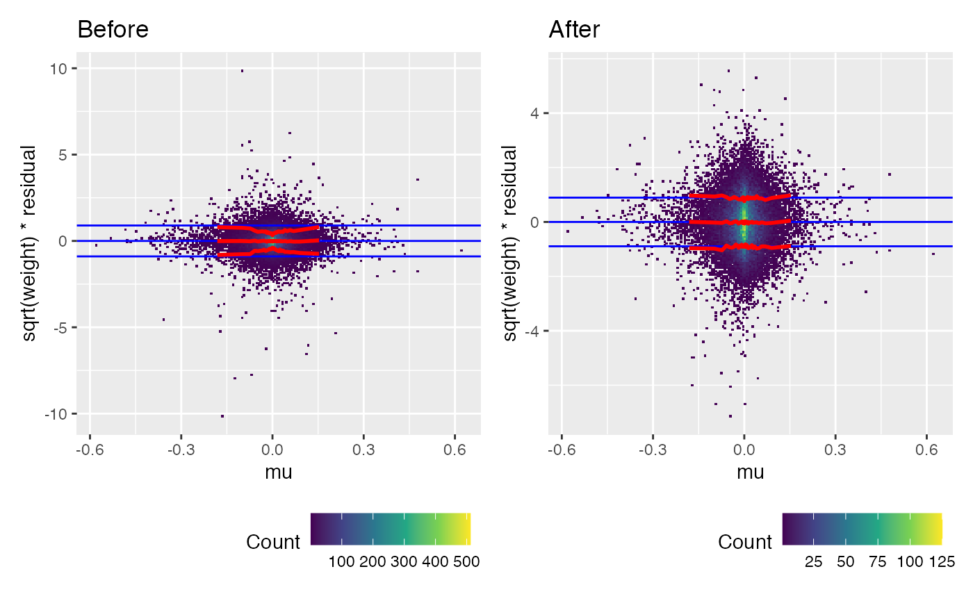
We can look at the calibration to per_read_var directly.
(weitrix_calplot(wei, comp, covar=per_read_var) + labs(title="Before")) +
(weitrix_calplot(cal_trend, comp, covar=per_read_var) + labs(title="After"))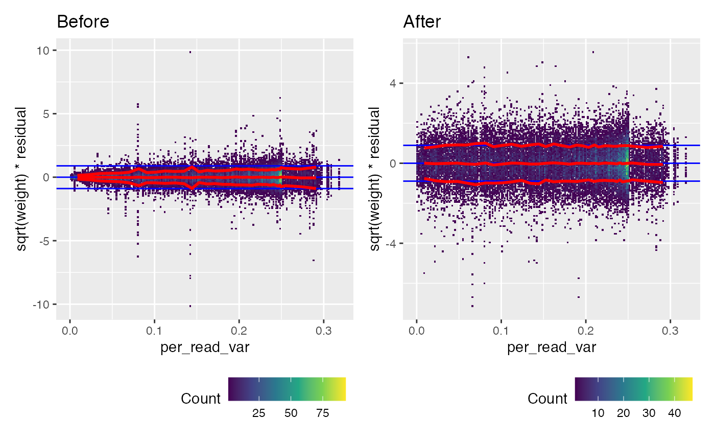
Weights were too large for large read counts. Calibration has applied a row-level adjustment for this based on the total number of reads for each row.
(weitrix_calplot(wei, comp, covar=log(weitrix_weights(wei))) + labs(title="Before")) +
(weitrix_calplot(cal_trend, comp, covar=log(weitrix_weights(wei))) + labs(title="After"))