5. SLAM-Seq proportion data example
Paul Harrison
2021-06-21
V5_slam_seq.Rmdweitrix is a jack of all trades. This vignette demonstrates the use of weitrix with proportion data. One difficulty is that when a proportion is exactly zero its variance should be exactly zero as well, leading to an infinite weight. To get around this, we slightly inflate the estimate of the variance for proportions near zero. This is not perfect, but calibration plots allow us to do this with our eyes open, and provide reassurance that it will not greatly interfere with downstream analysis.
We look at GSE99970, a SLAM-Seq experiment. In SLAM-Seq a portion of uracils are replaced with 4-thiouridine (s4U) during transcription, which by some clever chemistry leads to “T”s becoming “C”s in resultant RNA-Seq reads. The proportion of converted “T”s is an indication of the proportion of new transcripts produced while s4U was applied. In this experiment mouse embryonic stem cells were exposed to s4U for 24 hours, then washed out and sampled at different time points. The experiment lets us track the decay rates of transcripts.
library(tidyverse)
library(ComplexHeatmap)
library(weitrix)

# BiocParallel supports multiple backends.
# If the default hangs or errors, try others.
# The most reliable backed is to use serial processing
BiocParallel::register( BiocParallel::SerialParam() )
Load the data
The quantity of interest here is the proportion of “T”s converted to “C”s. We load the coverage and conversions, and calculate this ratio.
As an initial weighting, we use the coverage. Notionally, each proportion is an average of this many 1s and 0s. The more values averaged, the more accurate this is.
coverage <- system.file("GSE99970", "GSE99970_T_coverage.csv.gz", package="weitrix") %>%
    read_csv() %>%
    column_to_rownames("gene") %>%
    as.matrix()

conversions <- system.file("GSE99970", "GSE99970_T_C_conversions.csv.gz", package="weitrix") %>%
    read_csv() %>%
    column_to_rownames("gene") %>%
    as.matrix()

# Calculate proportions, create weitrix
wei <- as_weitrix( conversions/coverage, coverage )
dim(wei)
## [1] 22281 27
# We will only use genes where at least 30 conversions were observed
good <- rowSums(conversions) >= 30
wei <- wei[good,]

# Add some column data from the names
parts <- str_match(colnames(wei), "(.*)_(Rep_.*)")
colData(wei)$group <- fct_inorder(parts[,2])
colData(wei)$rep <- fct_inorder(paste0("Rep_",parts[,3]))
rowData(wei)$mean_coverage <- rowMeans(weitrix_weights(wei))

wei
## class: SummarizedExperiment
## dim: 11059 27
## metadata(1): weitrix
## assays(2): x weights
## rownames(11059): 0610005C13Rik 0610007P14Rik ... Zzef1 Zzz3
## rowData names(1): mean_coverage
## colnames(27): no_s4U_Rep_1 no_s4U_Rep_2 ... 24h_chase_Rep_2
## 24h_chase_Rep_3
## colData names(2): group rep## no_s4U_Rep_1 no_s4U_Rep_2 no_s4U_Rep_3 24h_s4U_Rep_1
## 0.0009467780 0.0008692730 0.0009657405 0.0228616995
## 24h_s4U_Rep_2 24h_s4U_Rep_3 0h_chase_Rep_1 0h_chase_Rep_2
## 0.0227623930 0.0224932745 0.0238126807 0.0233169898
## 0h_chase_Rep_3 0.5h_chase_Rep_1 0.5h_chase_Rep_2 0.5h_chase_Rep_3
## 0.0232719043 0.0223200231 0.0235324380 0.0231107497
## 1h_chase_Rep_1 1h_chase_Rep_2 1h_chase_Rep_3 3h_chase_Rep_1
## 0.0211553204 0.0216421689 0.0212003785 0.0138988066
## 3h_chase_Rep_2 3h_chase_Rep_3 6h_chase_Rep_1 6h_chase_Rep_2
## 0.0150091659 0.0149480630 0.0068880708 0.0072561156
## 6h_chase_Rep_3 12h_chase_Rep_1 12h_chase_Rep_2 12h_chase_Rep_3
## 0.0072943737 0.0022597908 0.0021795891 0.0021219205
## 24h_chase_Rep_1 24h_chase_Rep_2 24h_chase_Rep_3
## 0.0012122873 0.0010844372 0.0010793906Calibrate
We want to estimate the variance of each observation. We could model this exactly as each observed “T” encoded as 0 for unconverted and 1 for converted, having a Bernoulli distribution with a variance of \(\mu(1-\mu)\) for mean \(\mu\). The observed proportions are then an average of such values. For \(n\) such values, the variance of this average would be
\[ \sigma^2 = \frac{\mu(1-\mu)}{n} \]
However if our estimate of \(\mu\) is exactly zero, the variance would become zero and so the weight would become infinite. To avoid infinities:
- For calibration purposes, we ignore observations where the \(\mu\) is smaller than a certain value.
- We then assign weights based on clipping \(\mu\) to that value.
This is achieved using the mu_min argument to weitrix_calibrate_all. A natural choice to clip at is 0.001, the background rate of apparent T to C conversions seen due to sequencing errors.
A further possible problem is that biological variation does not disappear with greater and greater \(n\), so dividing by \(n\) may be over-optimistic. We will supply \(n\) (stored in weights) to a gamma GLM on the squared residuals with log link, using the Bernoulli variance as an offset. This GLM is then used to assign calibrated weights.
# Compute an initial fit to provide residuals
fit <- weitrix_components(wei, design=~group)

cal <- weitrix_calibrate_all(wei,
    design = fit,
    trend_formula =
        ~ log(weight) + offset(log(mu*(1-mu))),
    mu_min=0.001, mu_max=0.999)

metadata(cal)$weitrix$all_coef
## (Intercept) log(weight)
## 0.3391974 -0.9154304This trend formula was validated as adequate (although not perfect) by examining calibration plots, as demonstrated below.
The amount of conversion differs a great deal between timepoints, so we examine them individually.
weitrix_calplot(wei, fit, cat=group, covar=mu, guides=FALSE) +
    coord_cartesian(xlim=c(0,0.1)) + labs(title="Before calibration")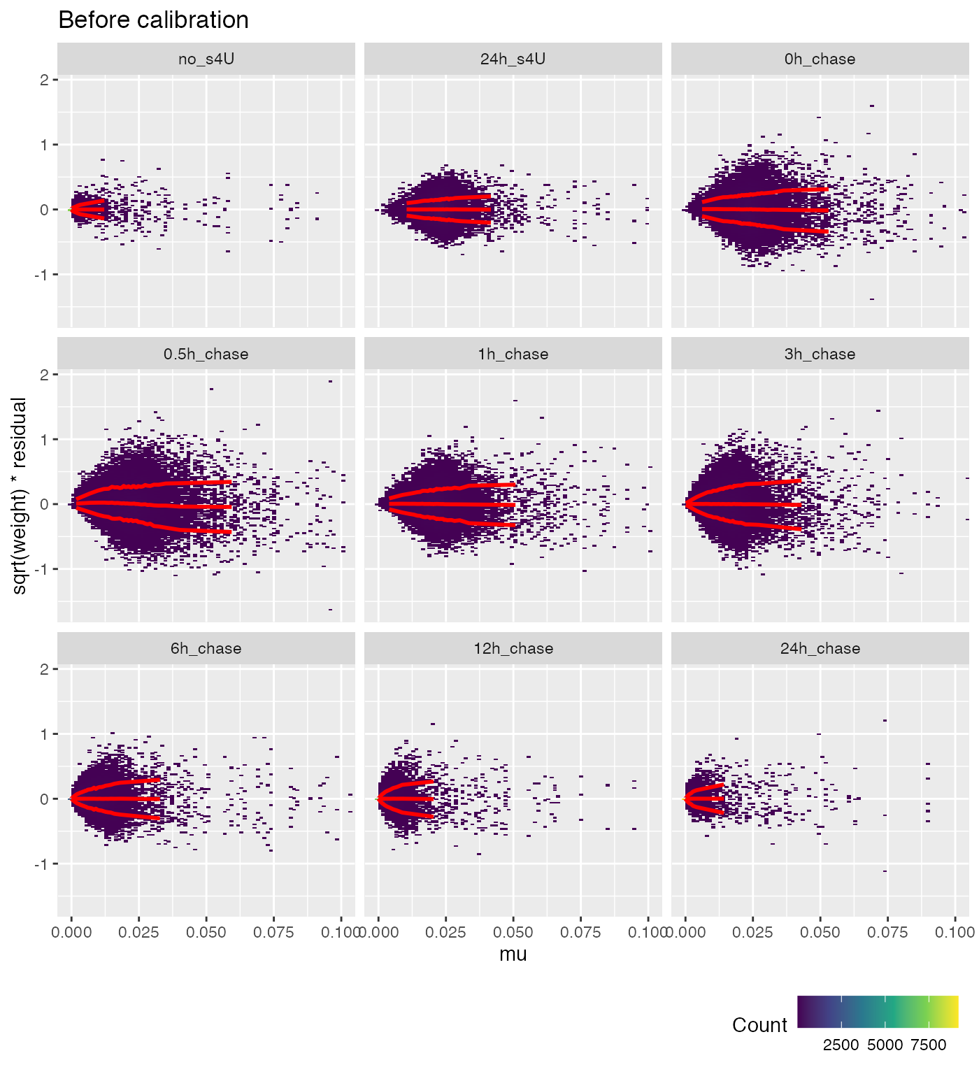
weitrix_calplot(cal, fit, cat=group, covar=mu) +
    coord_cartesian(xlim=c(0,0.1)) + labs(title="After calibration")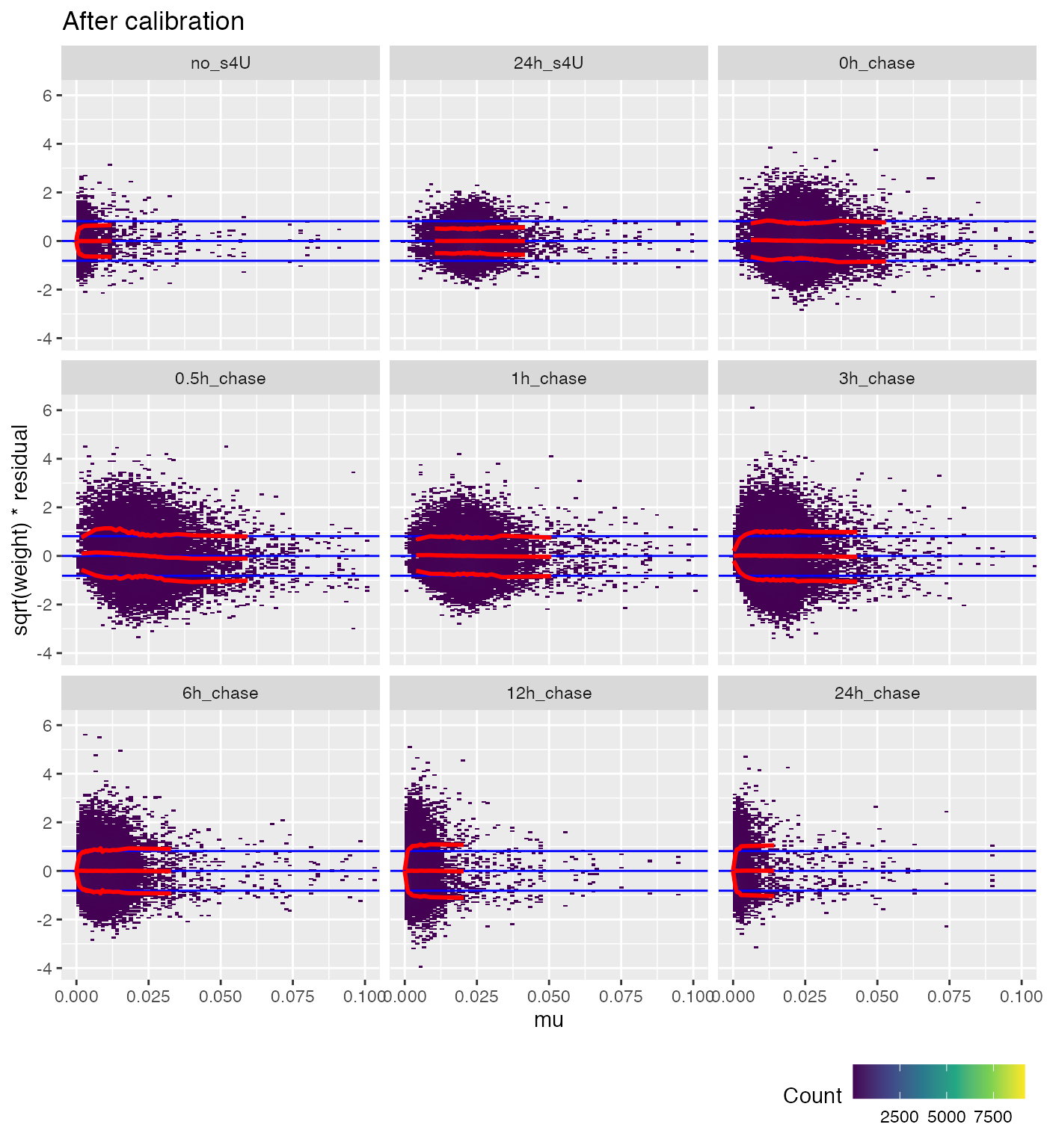
Ideally the red lines would all be horizontal. This isn’t possible for very small proportions, since this becomes a matter of multiplying zero by infinity.
We can also examine the weighted residuals vs the original weights (the coverage of “T”s).
weitrix_calplot(wei, fit, cat=group, covar=log(weitrix_weights(wei)), guides=FALSE) +
    labs(title="Before calibration")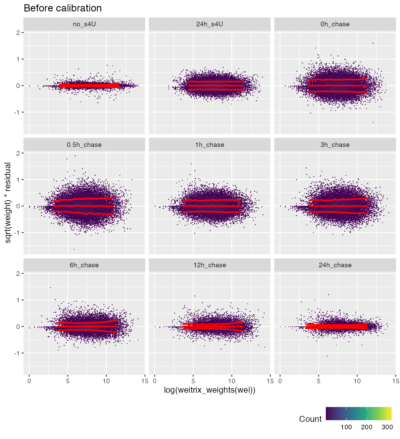
weitrix_calplot(cal, fit, cat=group, covar=log(weitrix_weights(wei))) +
    labs(title="After calibration")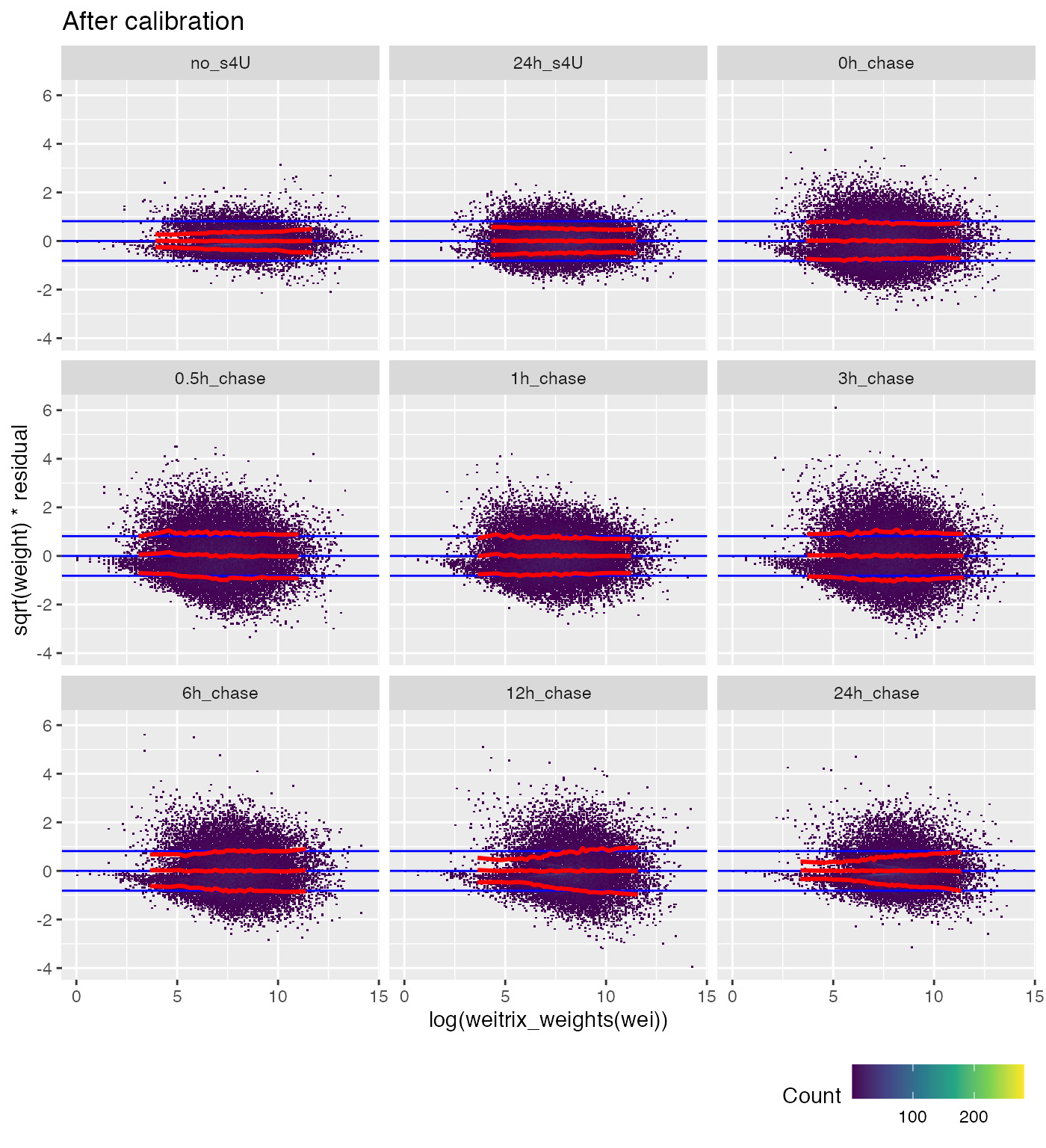
Components of variation
As a quick way to examine the data, we look for two components of variation. This reveals fast decaying and slow decaying genes.
comp <- weitrix_components(cal, 2, n_restarts=1)These are the scores for the two components:
matrix_long(comp$col[,-1], row_info=colData(cal)) %>%
    ggplot(aes(x=group,y=value)) +
    geom_jitter(width=0.2,height=0) +
    facet_grid(col~.)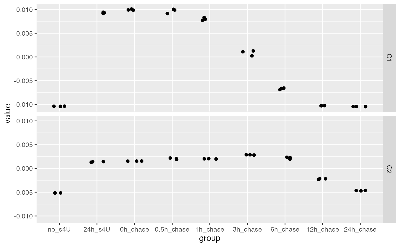
Component C1 highlights fast-decaying genes:
fast <- weitrix_confects(cal, comp$col, "C1")
fast
## $table
## confect effect se df fdr_zero row_mean typical_obs_err name
## 1 1.862 3.459 0.31563 41.46 2.789e-13 0.005283 0.0047807 Amd1
## 2 1.605 4.711 0.64117 41.46 1.018e-08 0.030215 0.0144486 Amd2
## 3 1.263 1.445 0.03834 41.46 3.932e-31 0.002195 0.0006714 Ifrd1
## 4 1.263 1.619 0.07678 41.46 1.649e-22 0.002626 0.0012189 Sap30
## 5 1.226 1.568 0.07489 41.46 2.097e-22 0.002113 0.0012066 Kifc1
## 6 1.225 1.417 0.04257 41.46 2.389e-29 0.002302 0.0006964 Dbf4
## 7 1.203 1.403 0.04479 41.46 2.101e-28 0.001949 0.0007577 Ccdc115
## 8 1.199 1.478 0.06347 41.46 5.418e-24 0.001844 0.0009379 Nfyc
## 9 1.199 1.327 0.02926 41.46 6.799e-34 0.001957 0.0004632 Cdk1
## 10 1.198 1.537 0.07797 41.46 1.617e-21 0.001620 0.0009991 Nr0b1
## mean_coverage
## 1 707.0
## 2 294.4
## 3 36516.7
## 4 5432.7
## 5 7994.1
## 6 31222.0
## 7 21676.3
## 8 8384.4
## 9 54062.4
## 10 12721.2
## ...
## 9956 of 11059 non-zero contrast at FDR 0.05
## Prior df 17.5
Heatmap(
    weitrix_x(cal)[ head(fast$table$name, 10) ,],
    name="Proportion converted",
    cluster_columns=FALSE, cluster_rows=FALSE)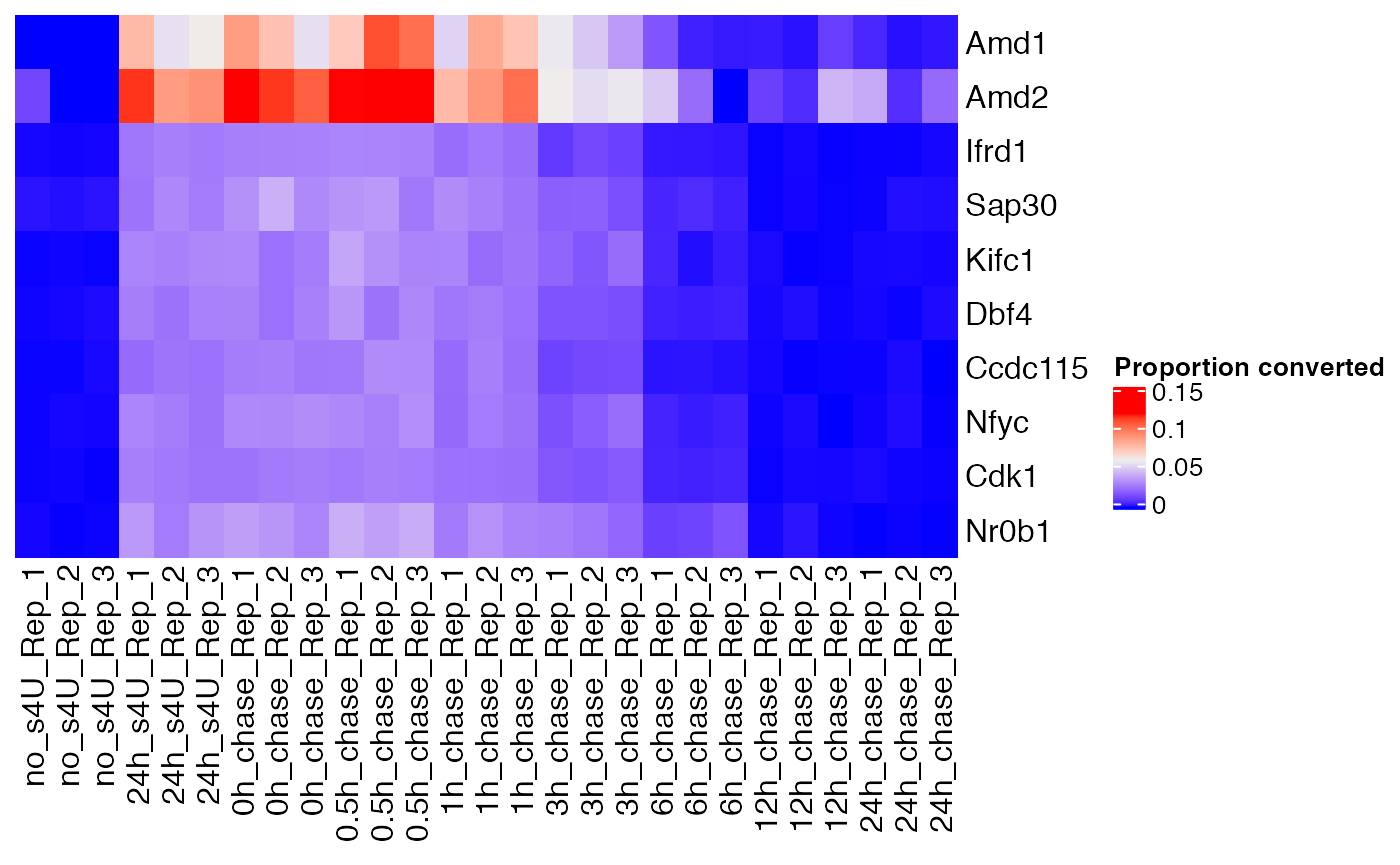
Component C2 highlights slow decaying genes:
slow <- weitrix_confects(cal, comp$col, "C2")
slow
## $table
## confect effect se df fdr_zero row_mean typical_obs_err name
## 1 3.187 7.919 0.9354 41.46 2.208e-09 0.038940 0.0096594 Morf4l1
## 2 2.530 5.590 0.6317 41.46 7.097e-10 0.007956 0.0037996 Rplp2
## 3 2.080 2.769 0.1461 41.46 5.000e-20 0.003845 0.0009094 Rpl27
## 4 2.026 2.629 0.1311 41.46 7.335e-21 0.003626 0.0008038 Cox5a
## 5 2.026 5.671 0.7999 41.46 1.452e-07 0.003747 0.0034680 Erh
## 6 2.010 3.092 0.2425 41.46 2.099e-14 0.004813 0.0016928 Snrpf
## 7 2.010 2.877 0.1962 41.46 2.553e-16 0.005089 0.0013151 Psmb2
## 8 2.010 7.485 1.2420 41.46 3.797e-06 0.002823 0.0039775 Pgk1
## 9 2.007 2.551 0.1244 41.46 3.492e-21 0.003584 0.0007722 Banf1
## 10 2.000 3.173 0.2713 41.46 2.842e-13 0.004837 0.0017907 Gm8624
## mean_coverage
## 1 887.8
## 2 2509.3
## 3 41892.9
## 4 61517.9
## 5 1871.4
## 6 12742.6
## 7 12790.4
## 8 959.0
## 9 50657.7
## 10 10490.3
## ...
## 3830 of 11059 non-zero contrast at FDR 0.05
## Prior df 17.5
Heatmap(
    weitrix_x(cal)[ head(slow$table$name, 10) ,],
    name="Proportion converted",
    cluster_columns=FALSE, cluster_rows=FALSE)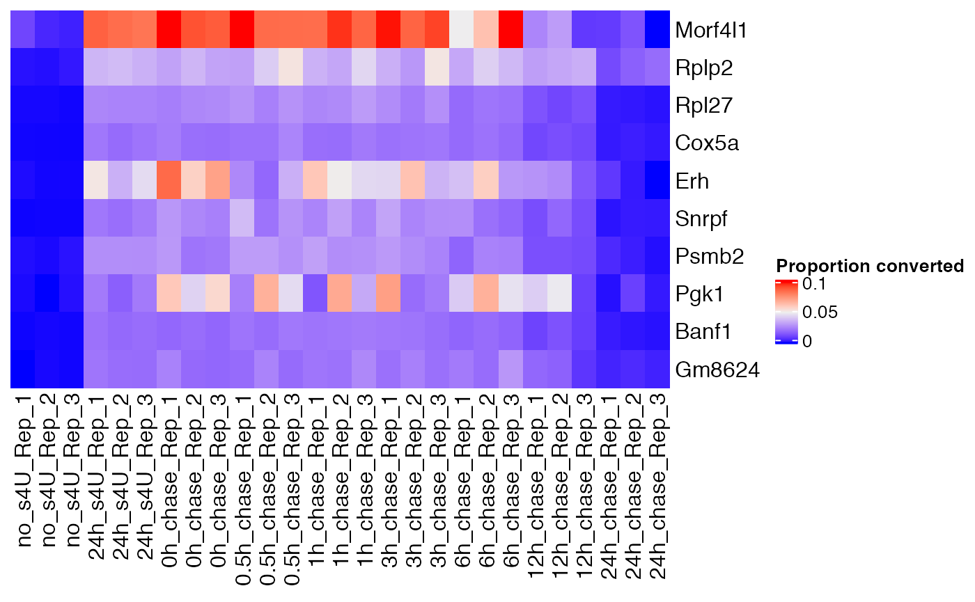
Further examination might be based on explicitly modelling the decay process.
Appendix: data download and extraction
Data was extracted and totalled into genes with:
library(tidyverse)

download.file("https://www.ncbi.nlm.nih.gov/geo/download/?acc=GSE99970&format=file", "GSE99970_RAW.tar")
untar("GSE99970_RAW.tar", exdir="GSE99970_RAW")

filenames <- list.files("GSE99970_RAW", full.names=TRUE)
samples <- str_match(filenames,"mESC_(.*)\\.tsv\\.gz")[,2]
dfs <- map(filenames, read_tsv, comment="#")
coverage <- do.call(cbind, map(dfs, "CoverageOnTs")) %>%
    rowsum(dfs[[1]]$Name)
conversions <- do.call(cbind, map(dfs, "ConversionsOnTs")) %>%
    rowsum(dfs[[1]]$Name)
colnames(conversions) <- colnames(coverage) <- samples

reorder <- c(1:3, 25:27, 4:24)

coverage[,reorder] %>%
    as.data.frame() %>%
    rownames_to_column("gene") %>%
    write_csv("GSE99970_T_coverage.csv.gz")

conversions[,reorder] %>%
    as.data.frame() %>%
    rownames_to_column("gene") %>%
    write_csv("GSE99970_T_C_conversions.csv.gz")