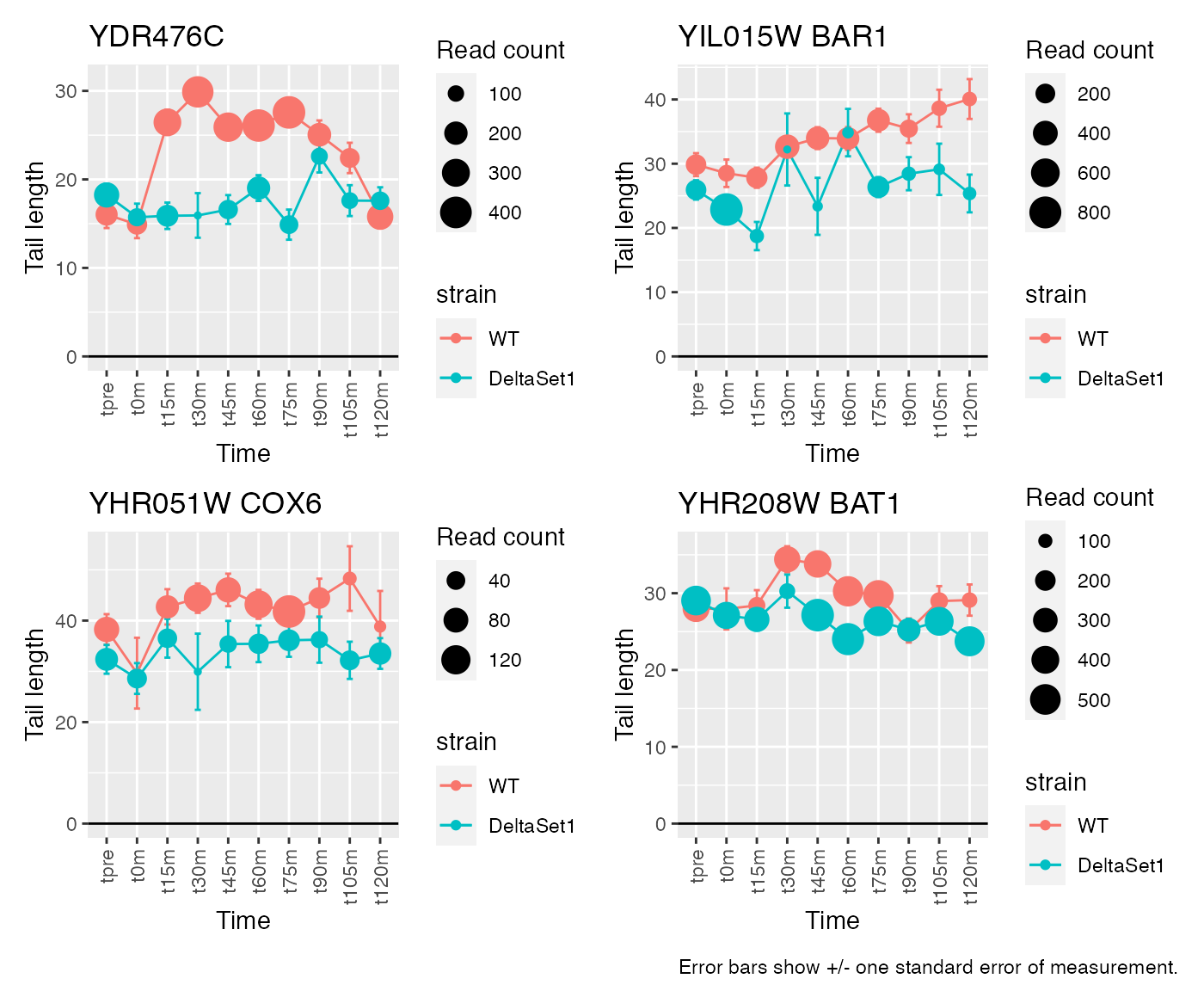
2. PAT-Seq poly(A) tail length example
Paul Harrison
2021-06-21
V2_tail_length.Rmdpoly(A) tail length of transcripts can be measured using the PAT-Seq protocol. This protocol produces 3’-end focussed reads that include the poly(A) tail. We examine GSE83162. This is a time-series experiment in which two strains of yeast are released into synchronized cell cycling and observed through two cycles. Yeast are treated with \(\alpha\)-factor, which causes them to stop dividing in antici… pation of a chance to mate. When the \(\alpha\)-factor is washed away, they resume cycling.
Read files, extract experimental design from sample names
library(tidyverse)     # ggplot2, etc
library(patchwork)     # side-by-side plots
library(limma)         # differential testing
library(topconfects)   # differential testing - top confident effect sizes
library(org.Sc.sgd.db) # Yeast organism info
library(weitrix)       # Matrices with precisions weights

# Produce consistent results
set.seed(12345)

# BiocParallel supports multiple backends.
# If the default hangs or errors, try others.
# The most reliable backed is to use serial processing
BiocParallel::register( BiocParallel::SerialParam() )
tail <- system.file("GSE83162", "tail.csv.gz", package="weitrix") %>%
    read_csv() %>%
    column_to_rownames("Feature") %>%
    as.matrix()

tail_count <- system.file("GSE83162", "tail_count.csv.gz", package="weitrix") %>%
    read_csv() %>%
    column_to_rownames("Feature") %>%
    as.matrix()

samples <- data.frame(sample=I(colnames(tail))) %>%
    extract(sample, c("strain","time"), c("(.+)-(.+)"), remove=FALSE) %>%
    mutate(
        strain=factor(strain,unique(strain)),
        time=factor(time,unique(time)))
rownames(samples) <- colnames(tail)

samples
## sample strain time
## WT-tpre WT-tpre WT tpre
## WT-t0m WT-t0m WT t0m
## WT-t15m WT-t15m WT t15m
## WT-t30m WT-t30m WT t30m
## WT-t45m WT-t45m WT t45m
## WT-t60m WT-t60m WT t60m
## WT-t75m WT-t75m WT t75m
## WT-t90m WT-t90m WT t90m
## WT-t105m WT-t105m WT t105m
## WT-t120m WT-t120m WT t120m
## DeltaSet1-tpre DeltaSet1-tpre DeltaSet1 tpre
## DeltaSet1-t0m DeltaSet1-t0m DeltaSet1 t0m
## DeltaSet1-t15m DeltaSet1-t15m DeltaSet1 t15m
## DeltaSet1-t30m DeltaSet1-t30m DeltaSet1 t30m
## DeltaSet1-t45m DeltaSet1-t45m DeltaSet1 t45m
## DeltaSet1-t60m DeltaSet1-t60m DeltaSet1 t60m
## DeltaSet1-t75m DeltaSet1-t75m DeltaSet1 t75m
## DeltaSet1-t90m DeltaSet1-t90m DeltaSet1 t90m
## DeltaSet1-t105m DeltaSet1-t105m DeltaSet1 t105m
## DeltaSet1-t120m DeltaSet1-t120m DeltaSet1 t120m“tpre” is the cells in an unsynchronized state, other times are minutes after release into cycling.
The two strains are a wildtype and a strain with a mutated set1 gene.
Create weitrix object
These tail lengths are each the average over many reads. We therefore weight each tail length by the number of reads. This is somewhat overoptimistic as there is biological noise that doesn’t go away with more reads, which we will correct for in the next step.
## good
## FALSE  TRUE
##  1657  4875
wei <- as_weitrix(
    tail[good,,drop=FALSE],
    weights=tail_count[good,,drop=FALSE])

rowData(wei)$gene <- AnnotationDbi::select(
    org.Sc.sgd.db, keys=rownames(wei), columns=c("GENENAME"))$GENENAME
rowData(wei)$total_reads <- rowSums(weitrix_weights(wei))
colData(wei) <- cbind(colData(wei), samples)
Calibration
Our first step is to calibrate our weights. Our weights are overoptimistic for large numbers of reads, as there is a biological components of noise that does not go away with more reads.
Calibration requires a model explaining non-random effects. We provide a design matrix and a weighted linear model fit is found for each row. The lack of replicates makes life difficult, for simplicity here we will assume time and strain are independent.
design <- model.matrix(~ strain + time, data=colData(wei))
fit <- weitrix_components(wei, design=design)
A gamma GLM with log link function can then be fitted to the squared residuals. 1 over the predictions from this models will serve as the new weights.
cal <- weitrix_calibrate_all(
    wei,
    design = fit,
    trend_formula = ~well_knotted_spline(mu,3)+well_knotted_spline(log(weight),3))
## mu range 4.402217 77.000000 knots 23.04834 30.07095 37.91549## log(weight) range 0.0000 10.6244 knots 2.841452 4.397124 6.359334For comparison, we’ll also look at completely unweighted residuals.
unwei <- wei
weitrix_weights(unwei) <- weitrix_weights(unwei) > 0
# (missing data still needs weight 0)
Calibration should remove any pattern in the weighted residuals, compared to known covariates. The trend line shown in red is based on the squared weighted residuals.
First look for any pattern relative to the linear model prediction (“mu”). A trend has been removed by the calibration.
weitrix_calplot(unwei, fit, covar=mu, guides=FALSE) + labs(title="Unweighted\n") |
weitrix_calplot(wei, fit, covar=mu, guides=FALSE) + labs(title="Weighted by\nread count") |
weitrix_calplot(cal, fit, covar=mu, guides=FALSE) + labs(title="Calibrated\n")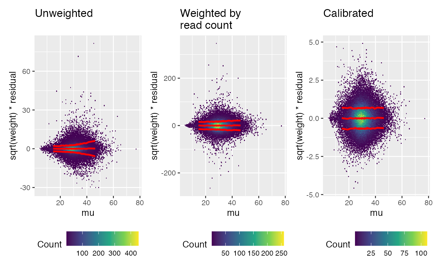
Next look for any pattern relative to the number of reads (recall these were the original weights). Again, a trend has been removed by the calibration.
weitrix_calplot(unwei, fit, covar=log(weitrix_weights(wei)), guides=FALSE) + labs(title="Unweighted\n") |
weitrix_calplot(wei, fit, covar=log(weitrix_weights(wei)), guides=FALSE) + labs(title="Weighted by\nread count") |
weitrix_calplot(cal, fit, covar=log(weitrix_weights(wei)), guides=FALSE) + labs(title="Calibrated\n")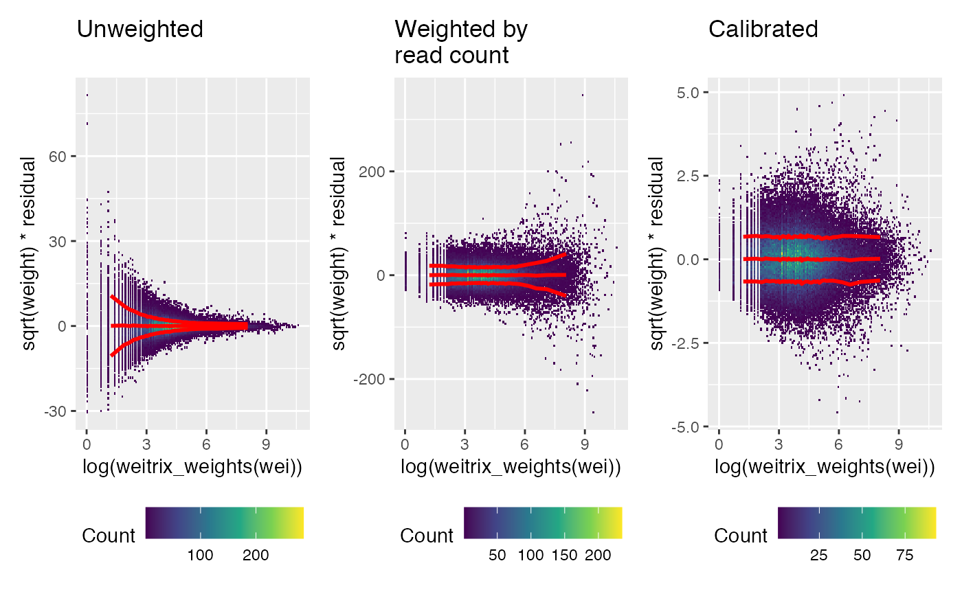
Testing
Top confident effects
We are now ready to test things.
My recommended approach is to find top confident effects, here top confident differential tail length. Core functionality is implemented in my package topconfects. Applying this to a weitrix is done using the weitrix_confects function. Rather than picking “most significant” genes, it will highlight genes with a large effect size.
weitrix_confects(cal, design, coef="strainDeltaSet1", fdr=0.05)## $table
## confect effect se df fdr_zero row_mean typical_obs_err
## 1 -2.569 -6.027 0.6864 30.25 3.915e-06 26.23 1.485
## 2 -2.104 -7.124 1.0472 30.25 3.538e-04 29.08 2.057
## 3 -1.212 -5.070 0.8298 30.25 1.207e-03 14.87 1.773
## 4 -1.064 -3.420 0.5180 30.25 4.108e-04 19.10 1.119
## 5 -0.872 -3.470 0.5833 30.25 1.265e-03 20.29 1.267
## 6 -0.872 -7.505 1.5042 30.25 6.497e-03 38.19 3.062
## 7 -0.872 -3.304 0.5610 30.25 1.279e-03 18.36 1.218
## 8 -0.872 -6.710 1.3544 30.25 6.497e-03 20.48 2.627
## 9 -0.831 -2.867 0.4782 30.25 1.265e-03 26.88 1.055
## 10 0.828 5.472 1.0990 30.25 6.497e-03 29.08 2.290
## name gene total_reads
## 1 YDR170W-A <NA> 4832
## 2 YIL015W BAR1 3898
## 3 YAR009C <NA> 1866
## 4 YJR027W/YJR026W <NA> 6577
## 5 YML045W/YML045W-A <NA> 4553
## 6 YHR051W COX6 1167
## 7 YPL257W-B/YPL257W-A <NA> 5729
## 8 YOR192C-B/YOR192C-A <NA> 864
## 9 YIL053W GPP1 25996
## 10 YGL209W MIG2 1937
## ...
## 112 of 4875 non-zero contrast at FDR 0.05
## Prior df 21.2This lists the largest confident changes in poly(A) tail length. The confect column is an inner confidence bound on the difference in tail length, adjusted for multiple testing.
Note that due to PCR amplification slippage and limited read length, the observed poly(A) tail lengths may be an underestimate. However as all samples have been prepared in the same way, observed differences should indicate the existence of true differences.
If you prefer to rank by signal to noise ratio, it is possible to use Cohen’s f as an effect size. This is similar to ranking by p-value, but Cohen’s f can be interpreted meaningfully as a signal to noise ratio.
weitrix_confects(cal, design, coef="strainDeltaSet1", effect="cohen_f", fdr=0.05)## $table
## confect effect strainDeltaSet1 fdr_zero row_mean typical_obs_err
## 1 0.569 1.963 -6.027 3.915e-06 26.23 1.4851
## 2 0.322 1.521 -7.124 3.538e-04 29.08 2.0570
## 3 0.317 1.476 -3.420 4.108e-04 19.10 1.1193
## 4 0.259 1.366 -5.070 1.207e-03 14.87 1.7733
## 5 0.259 1.341 -2.867 1.265e-03 26.88 1.0552
## 6 0.259 1.330 -3.470 1.265e-03 20.29 1.2672
## 7 0.259 1.317 -3.304 1.279e-03 18.36 1.2180
## 8 0.174 1.190 -2.846 5.584e-03 18.31 1.1618
## 9 0.171 1.170 -2.804 6.426e-03 18.99 1.1637
## 10 0.171 1.144 -2.283 6.497e-03 27.95 0.9934
## name gene total_reads
## 1 YDR170W-A <NA> 4832
## 2 YIL015W BAR1 3898
## 3 YJR027W/YJR026W <NA> 6577
## 4 YAR009C <NA> 1866
## 5 YIL053W GPP1 25996
## 6 YML045W/YML045W-A <NA> 4553
## 7 YPL257W-B/YPL257W-A <NA> 5729
## 8 YLR157C-B/YLR157C-A <NA> 5519
## 9 YPR137C-B/YPR137C-A <NA> 7287
## 10 YOL109W ZEO1 34839
## ...
## 112 of 4875 non-zero Cohen's f at FDR 0.05
## Prior df 21.2Testing with limma
If you prefer a more traditional approach, we can feed our calibrated weitrix to limma.
fit_cal_design <- cal %>%
    weitrix_elist() %>%
    lmFit(design)

ebayes_fit <- eBayes(fit_cal_design)

topTable(ebayes_fit, "strainDeltaSet1", n=10) %>%
    dplyr::select(
        gene,diff_tail=logFC,ave_tail=AveExpr,adj.P.Val,total_reads)
## gene diff_tail ave_tail adj.P.Val total_reads
## YDR170W-A <NA> -6.027208 25.87662 3.915262e-06 4832
## YJR027W/YJR026W <NA> -3.419778 19.40928 4.107986e-04 6577
## YIL015W BAR1 -7.124118 30.24503 3.538329e-04 3898
## YAR009C <NA> -5.070438 15.56624 1.207189e-03 1866
## YIL053W GPP1 -2.867498 27.19599 1.265338e-03 25996
## YML045W/YML045W-A <NA> -3.470070 20.55073 1.265338e-03 4553
## YPL257W-B/YPL257W-A <NA> -3.304377 18.59545 1.278512e-03 5729
## YLR157C-B/YLR157C-A <NA> -2.845888 18.46280 5.584245e-03 5519
## YPR137C-B/YPR137C-A <NA> -2.803791 19.21016 6.425669e-03 7287
## YOL109W ZEO1 -2.282940 28.11748 6.497358e-03 34839Testing multiple contrasts
weitrix_confects can also be used as an omnibus test of multiple contrasts. Here the default effect size will be standard deviation of observations explained by the part of the model captured by the contrasts. The standardized effect size “Cohen’s f” can also be used.
Here we will look for any step changes between time steps, ignoring the “tpre” timepoint. The exact way these contrasts are specified will not modify the ranking, so long as they specify the same subspace of coefficients.
multiple_contrasts <- limma::makeContrasts(
    timet15m-timet0m, timet30m-timet15m, timet45m-timet30m,
    timet60m-timet45m,  timet75m-timet60m, timet90m-timet75m,
    timet105m-timet90m, timet120m-timet105m,
    levels=design)
## Warning in limma::makeContrasts(timet15m - timet0m, timet30m - timet15m, :
## Renaming (Intercept) to Intercept
weitrix_confects(cal, design, contrasts=multiple_contrasts, fdr=0.05)## $table
## confect effect timet15m - timet0m timet30m - timet15m timet45m - timet30m
## 1 3.5 5.858 -9.8373 10.8696 1.5141
## 2 3.5 7.524 -0.3369 -0.3586 8.7815
## 3 3.5 5.785 -0.4785 4.0872 -2.2867
## 4 3.5 5.323 -6.8395 10.2452 0.8396
## 5 3.4 7.410 -11.8301 7.4880 4.4171
## 6 3.2 9.821 -8.3607 7.6550 18.4197
## 7 2.8 6.285 -6.8300 10.1441 6.2579
## 8 2.8 4.078 4.8376 -7.2995 -3.3326
## 9 2.7 7.400 2.3901 6.4600 -0.1309
## 10 2.6 3.722 2.6153 1.9706 -0.3507
## timet60m - timet45m timet75m - timet60m timet90m - timet75m
## 1 -0.1804 1.857 -1.2957
## 2 -0.4211 12.594 -5.5116
## 3 7.2778 8.972 -1.4281
## 4 0.1190 5.537 -2.5875
## 5 7.2070 1.792 -5.5915
## 6 -13.1018 18.661 -13.1212
## 7 -2.3809 4.930 -5.4150
## 8 -0.1799 5.257 4.4367
## 9 3.7622 11.352 -15.9122
## 10 2.4888 3.903 0.1883
## timet105m - timet90m timet120m - timet105m fdr_zero row_mean
## 1 3.97229 -0.40015 2.440e-08 29.37
## 2 3.86528 0.20344 6.670e-06 45.91
## 3 -0.07182 -1.28441 1.210e-07 30.67
## 4 1.64288 -1.47056 1.231e-08 38.24
## 5 0.76415 -0.79431 1.661e-05 29.85
## 6 -2.41187 7.39443 2.320e-04 31.90
## 7 2.28033 -2.57263 2.771e-05 36.33
## 8 1.34827 0.02541 1.774e-09 14.49
## 9 14.50129 -5.28822 2.028e-04 39.64
## 10 1.16199 -1.69823 1.774e-09 22.41
## typical_obs_err name gene total_reads
## 1 1.833 YNL036W NCE103 5712
## 2 3.156 YBL097W BRN1 1680
## 3 1.960 YBL016W FUS3 6287
## 4 1.604 YKR093W PTR2 23012
## 5 3.280 YHL021C AIM17 793
## 6 5.191 YDL204W RTN2 418
## 7 2.885 YML100W TSL1 1780
## 8 1.124 YFL014W HSP12 9509
## 9 3.862 YER185W PUG1 813
## 10 1.013 YOR096W RPS7A 72660
## ...
## 511 of 4875 non-zero standard deviation explained at FDR 0.05
## Prior df 21.2Examine individual genes
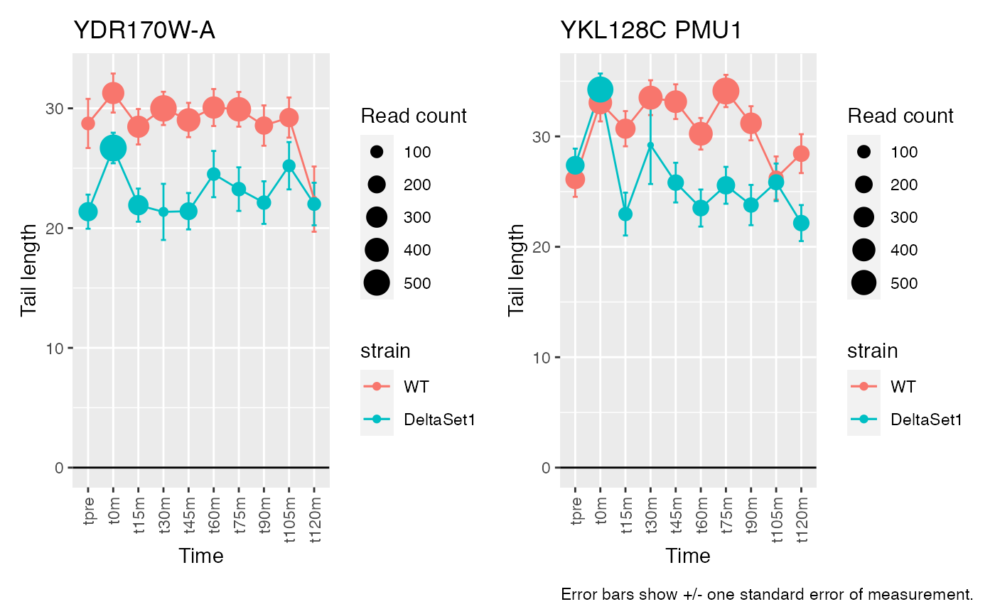
Having discovered genes with differential tail length, let’s look at some genes in detail.
view_gene <- function(id) {
    gene <- rowData(wei)[id,"gene"]
    if (is.na(gene)) gene <- ""
    tails <- weitrix_x(cal)[id,]
    std_errs <- weitrix_weights(cal)[id,] ^ -0.5
    ggplot(samples) +
        aes(x=time,color=strain,group=strain,
            y=tails, ymin=tails-std_errs, ymax=tails+std_errs) +
        geom_errorbar(width=0.2) +
        geom_hline(yintercept=0) +
        geom_line() +
        geom_point(aes(size=tail_count[id,])) +
        labs(x="Time", y="Tail length", size="Read count", title=paste(id,gene)) +
        theme(axis.text.x=element_text(angle=90, hjust=1, vjust=0.5))
}

caption <- plot_annotation(
    caption="Error bars show +/- one standard error of measurement.")

# Top confident differences between WT and deltaSet1
view_gene("YDR170W-A") +
view_gene("YIL015W") +
view_gene("YAR009C") +
view_gene("YJR027W/YJR026W") +
caption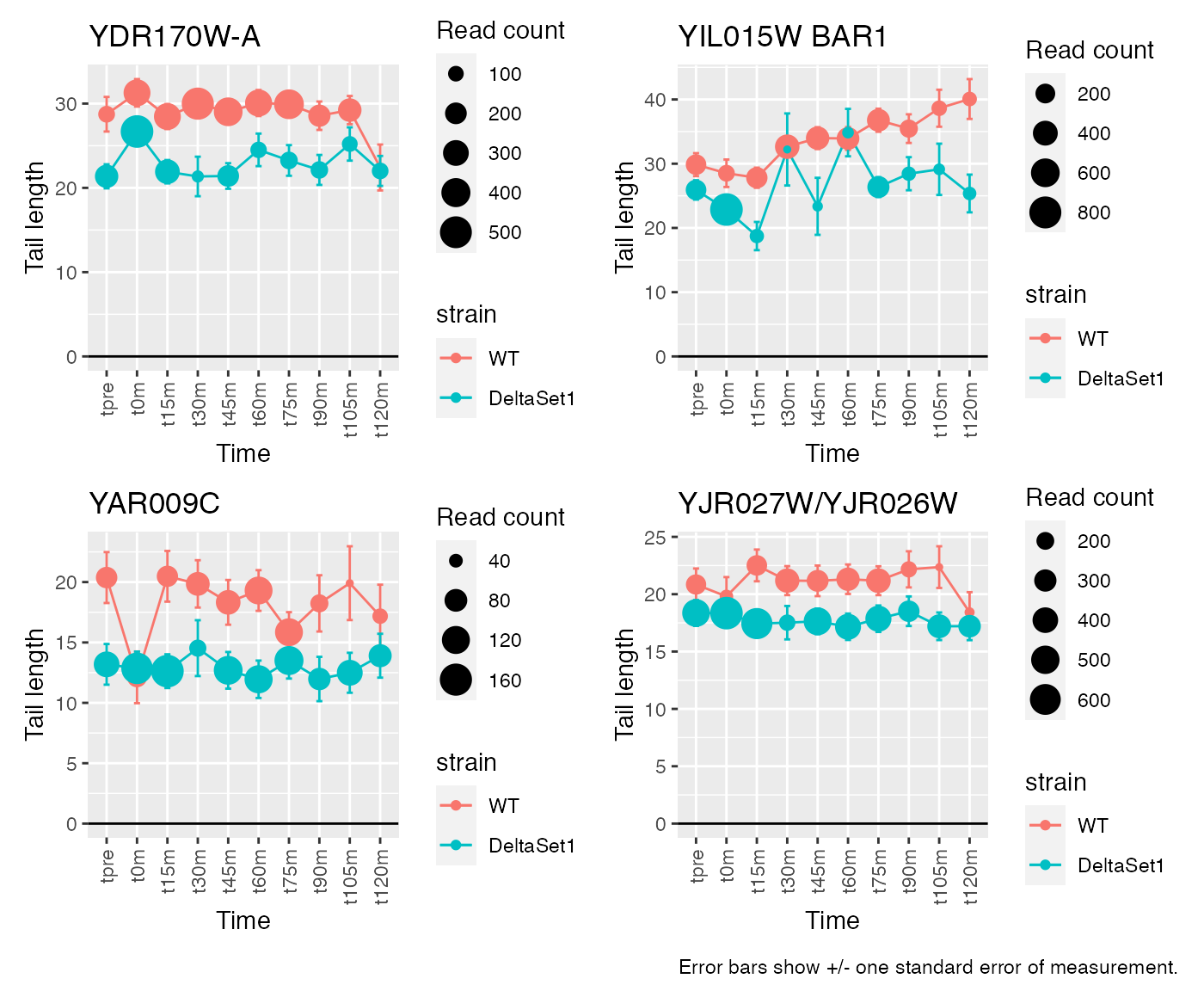
# Top confident changes over time
view_gene("YNL036W") +
view_gene("YBL097W") +
view_gene("YBL016W") +
view_gene("YKR093W") +
caption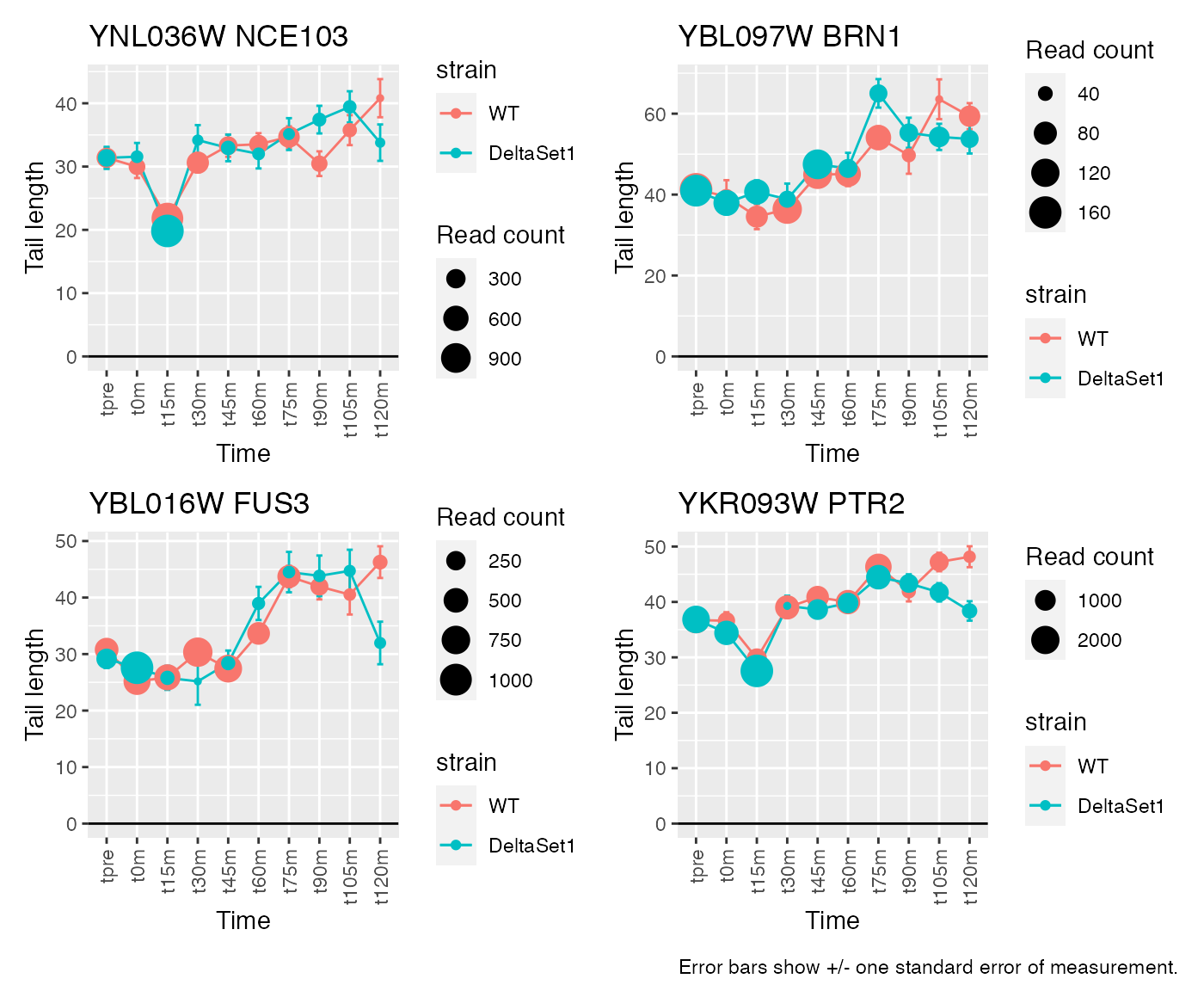
Exploratory analysis: overdispersed genes
Genes with high dispersion (weighted residual variance) may be of biological interest. Here we examine dispersion relative to a simple model with only an intercept term. When the dispersion is greater than 1, there is variation in excess of that expected from our calibrated weights. The function weitrix_dispersions can be used to calculate dispersions.
To make this a bit more concrete, we can estimate how much extra variation there is per observation not explained by the model. The function weitrix_sd_confects provides this, and further provides a confident lower bound on this excess with a multiple testing correction. The “effect” column in the output is excess variation, and the “confect” column is a confident lower bound on this. Results are sorted by confect. These effects are in the same units as the observations themselves. They can be interpreted as the standard deviation if there was no observational error.
confects <- weitrix_sd_confects(cal, ~1)
confects
## $table
## confect effect row_mean typical_obs_err dispersion n_present df fdr_zero
## 1 4.714 7.857 45.91 3.092 7.456 20 19 0.000e+00
## 2 4.499 9.792 31.90 5.157 4.605 20 19 3.869e-09
## 3 4.354 6.001 29.37 1.761 12.608 20 19 0.000e+00
## 4 4.274 5.624 38.24 1.486 15.325 20 19 0.000e+00
## 5 4.274 5.910 30.67 1.804 11.739 20 19 0.000e+00
## 6 4.172 7.278 26.52 3.258 5.989 19 18 5.567e-13
## 7 3.904 4.999 32.85 1.243 17.182 20 19 0.000e+00
## 8 3.830 6.396 36.33 2.826 6.123 20 19 4.163e-14
## 9 3.739 5.754 30.83 2.267 7.443 20 19 0.000e+00
## 10 3.730 4.938 29.33 1.398 13.471 20 19 0.000e+00
## name gene total_reads
## 1 YBL097W BRN1 1680
## 2 YDL204W RTN2 418
## 3 YNL036W NCE103 5712
## 4 YKR093W PTR2 23012
## 5 YBL016W FUS3 6287
## 6 YIL082W-A/YIL082W <NA> 842
## 7 YDR461W MFA1 83042
## 8 YML100W TSL1 1780
## 9 YMR105C PGM2 2616
## 10 YCL042W/YCL040W <NA> 12370
## ...
## 745 of 4875 non-zero excess standard deviation at FDR 0.05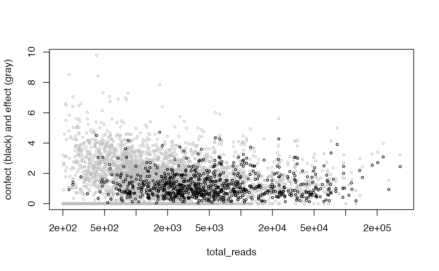
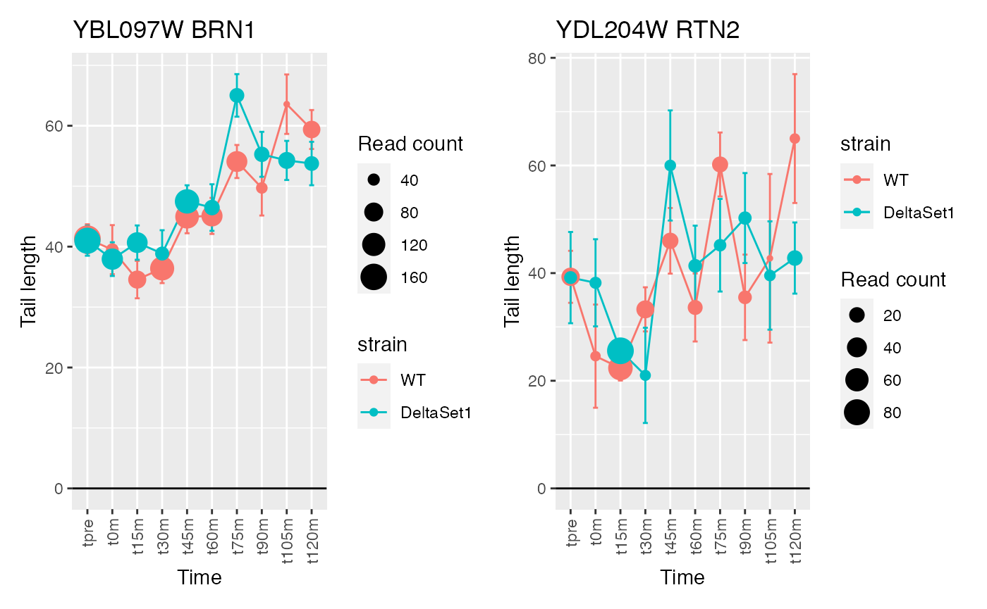
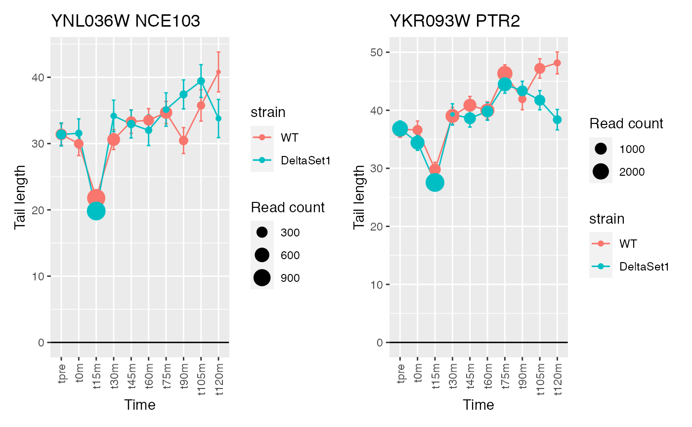
## Warning: Removed 1 row(s) containing missing values (geom_path).## Warning: Removed 1 rows containing missing values (geom_point).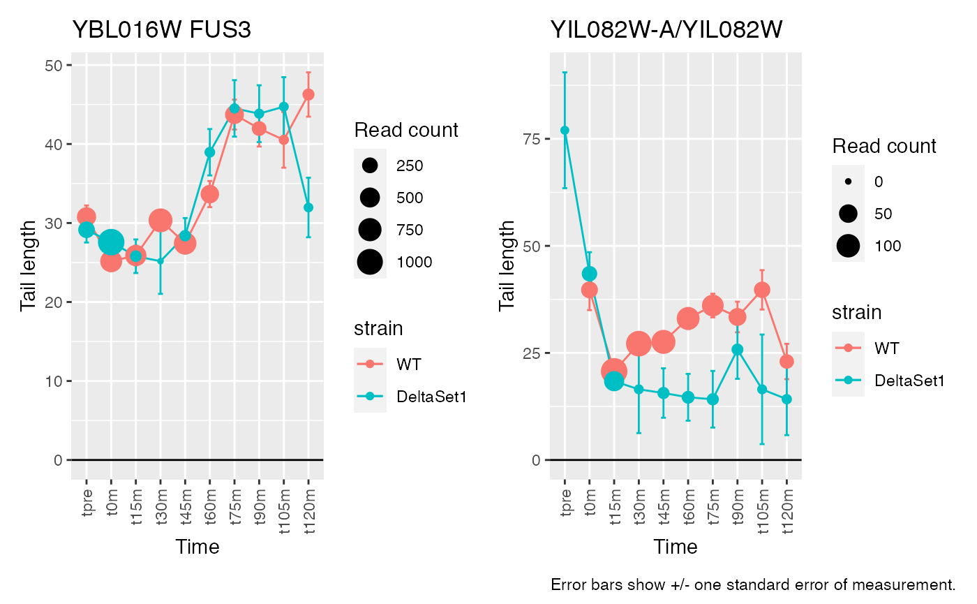
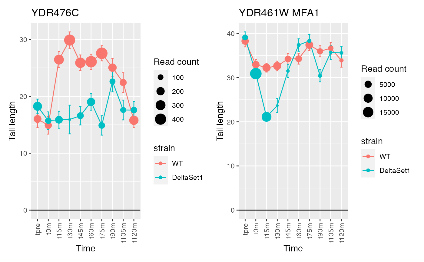
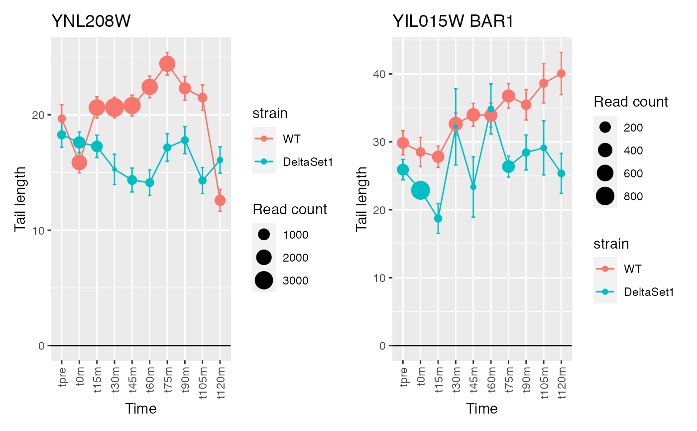
The genes discovered tend to be changing over time. If we use a model that accounts for time, differences between the two strains will be emphasized instead.
confects2 <- weitrix_sd_confects(cal, ~time)
confects2
## $table
## confect effect row_mean typical_obs_err dispersion n_present df fdr_zero
## 1 3.018 5.094 20.61 1.516 12.299 20 10 0.000e+00
## 2 2.289 3.933 32.85 1.243 11.018 20 10 0.000e+00
## 3 2.259 3.571 18.35 1.022 13.214 20 10 0.000e+00
## 4 2.002 4.590 29.08 1.974 6.403 20 10 4.325e-07
## 5 1.905 3.995 26.23 1.631 7.001 20 10 5.374e-08
## 6 1.639 3.773 28.75 1.665 6.135 20 10 1.089e-06
## 7 1.531 3.173 31.76 1.309 6.877 20 10 7.457e-08
## 8 1.528 3.514 34.39 1.576 5.971 20 10 2.003e-06
## 9 1.209 2.616 25.12 1.133 6.329 20 10 5.250e-07
## 10 1.175 4.000 40.16 2.166 4.410 20 10 5.930e-04
## name gene total_reads
## 1 YDR476C <NA> 4196
## 2 YDR461W MFA1 83042
## 3 YNL208W <NA> 23220
## 4 YIL015W BAR1 3898
## 5 YDR170W-A <NA> 4832
## 6 YKL128C PMU1 5443
## 7 YBR009C HHF1 33533
## 8 YDR224C HTB1 13374
## 9 YMR295C <NA> 20878
## 10 YOL092W YPQ1 4661
## ...
## 89 of 4875 non-zero excess standard deviation at FDR 0.05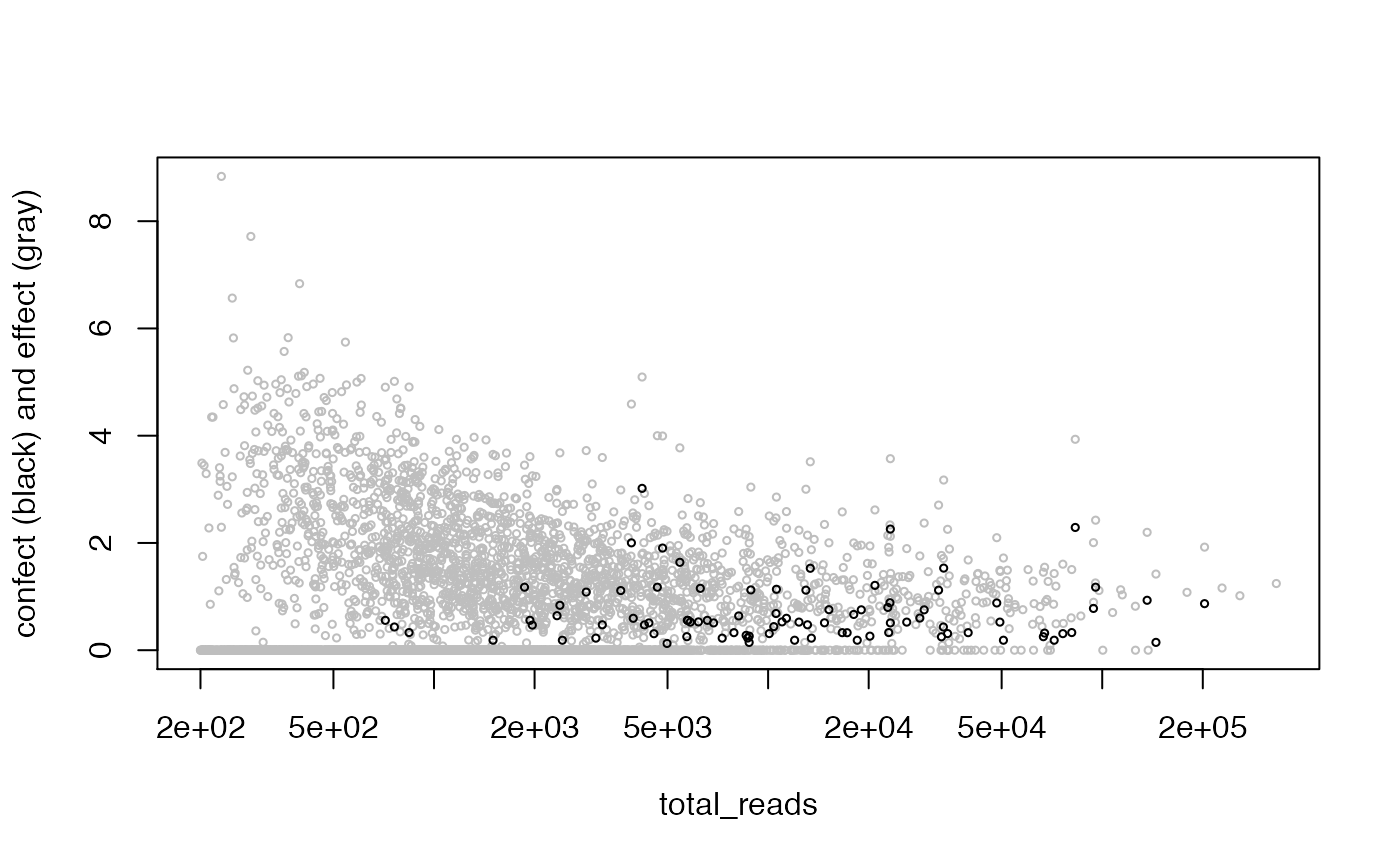
Exploratory analysis: components of variation
The test we’ve performed was somewhat unsatisfactory. Due to the design of the experiment it’s difficul to specify differential tests that fully interrogate this dataset: the lack of replicates, and the difficult specifying apriori how tail length will change over time.
Perhaps we should let the data speak for itself.
Perhaps this is what we should have done first!
The weitrix package allows us to look for components of variation. We’ll try to explain the data with different numbers of components (from 1 to 6 components).
comp_seq <- weitrix_components_seq(cal, p=6)weitrix_seq_screeplot shows how much additional variation in the data is explained as each further component is allowed. However the ultimate decision of how many components to examine is a matter of judgement.
components_seq_screeplot(comp_seq)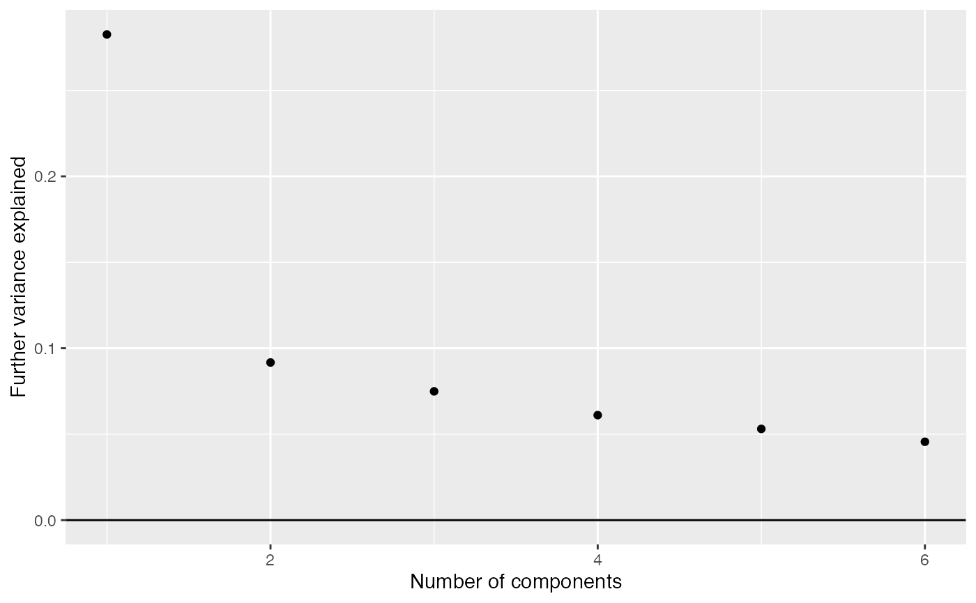
Looking at three components shows some of the major trends in this data-set.
comp <- comp_seq[[3]]

matrix_long(comp$col[,-1], row_info=samples, varnames=c("sample","component")) %>%
    ggplot(aes(x=time, y=value, color=strain, group=strain)) +
    geom_hline(yintercept=0) +
    geom_line() +
    geom_point(alpha=0.75, size=3) +
    facet_grid(component ~ .) +
    labs(title="Sample scores for each component", y="Sample score", x="Time", color="Strain")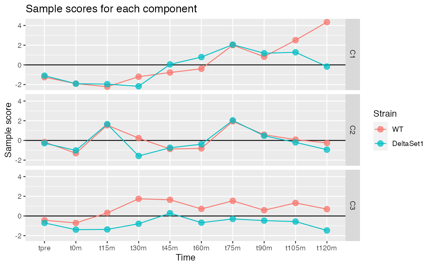
We observe:
- C1 - A gradual lengthening of tails after release into cell cycling. (The reason for the divergence between strains at the end is unclear.)
- C2 - Variation in poly(A) tail length with the cell cycle.
- C3 - A lengthening of poly(A) tails in the set1 mutant.
The tail lengths are approximated by comp$row %*% t(comp$col) where comp$col is an \(n_\text{sample} \times (p+1)\) matrix of scores (shown above), and comp$row is an \(n_\text{gene} \times (p+1)\) matrix of gene loadings, which we will now examine. (The \(+1\) is the intercept “component”, allowing each gene to have a different baseline tail length.)
Treat these results with caution. Confindence bounds take into account uncertainty in the loadings but not in the scores! What follows is best regarded as exploratory rather than a final result.
Gene loadings for C1: gradual lengthing over time
result_C1 <- weitrix_confects(cal, comp$col, coef="C1")## gene loading confect total_reads
## 1 BRN1 4.657827 2.466 1680
## 2 FUS3 3.943944 2.364 6287
## 3 RTN2 6.397080 2.327 418
## 4 TBS1 3.432363 1.975 2872
## 5 PGM2 3.561471 1.887 2616
## 6 AIM17 4.139319 1.675 793
## 7 TSL1 3.257115 1.675 1780
## 8 <NA> 2.653402 1.660 12370
## 9 <NA> 3.388808 1.655 2342
## 10 PTR2 2.672167 1.655 23012## 1100 genes significantly non-zero at FDR 0.05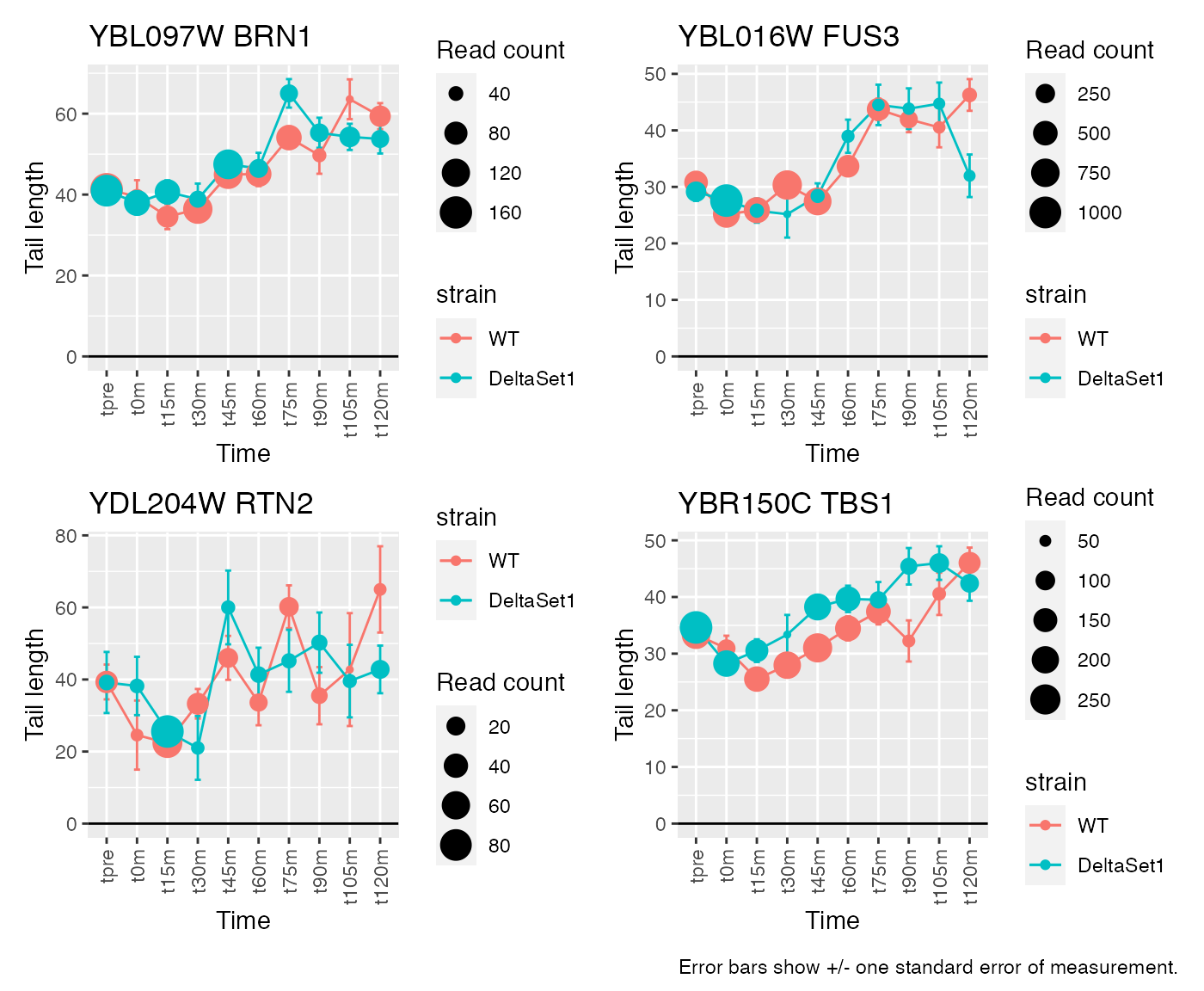
FUS3 is involved in yeast mating. We see here a poly(A) tail signature of yeast realizing there are not actually any \(\alpha\) cells around to mate with.
Gene loadings for C2: cell-cycle associated changes
result_C2 <- weitrix_confects(cal, comp$col, coef="C2")## gene loading confect total_reads
## 1 MSH6 5.363888 1.894 996
## 2 RFA3 4.056017 1.894 3963
## 3 CDC21 5.095419 1.853 1268
## 4 TOS6 4.633834 1.853 4024
## 5 NCE103 -3.111051 -1.464 5712
## 6 GAS1 2.794274 1.464 49500
## 7 RNR1 3.483311 1.353 5659
## 8 SVS1 3.660240 1.353 11347
## 9 <NA> 3.156380 1.283 12356
## 10 HSL1 3.364123 1.096 3676## 205 genes significantly non-zero at FDR 0.05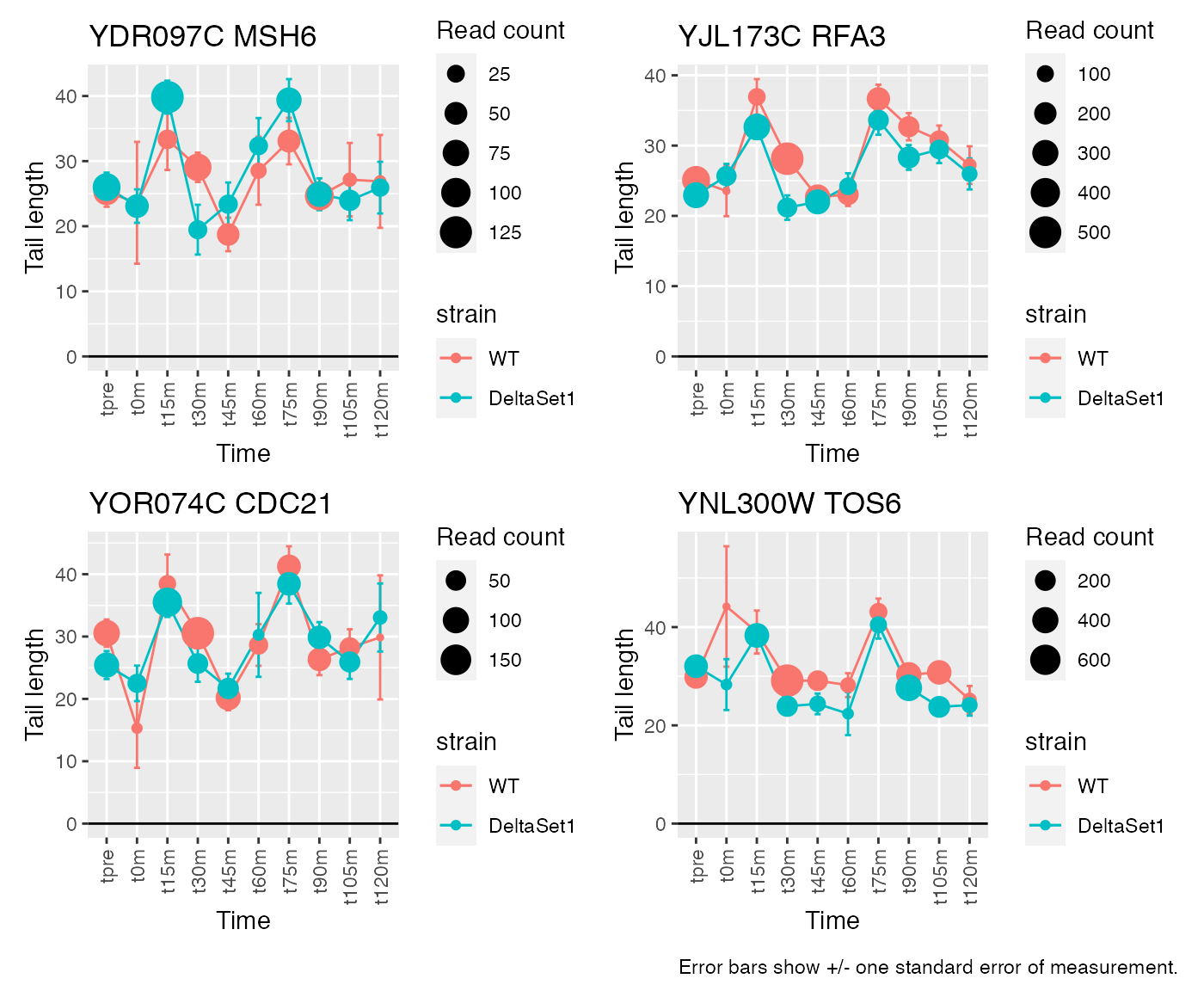
Gene loadings for C3: longer tails in set1 mutant
result_C3 <- weitrix_confects(cal, comp$col, coef="C3")Given the mixture of signs for effects in C3, different genes are longer in different stages of the cell cycle. We see many genes to do with replication.
##      gene  loading confect total_reads
## 1    <NA> 4.162831   1.653        4196
## 2    BAR1 3.640595   1.548        3898
## 3    COX6 4.316285   1.262        1167
## 4    BAT1 2.448882   0.899        6868
## 5    POL4 4.210052   0.875         606
## 6    RPP0 1.801468   0.746       25545
## 7    SSB2 1.756091   0.743       17238
## 8    RPL5 1.662335   0.734       81051
## 9  RPL21B 1.860615   0.713       23159
## 10 RPL12B 1.458424   0.569       34361
## 347 genes significantly non-zero at FDR 0.05