Natural cubic spline with good choice of knots
well_knotted_spline.RdFor use in model formulas,
natural cubic spline as in splines::ns
but with knot positions chosen using
k-means rather than quantiles.
Automatically uses less knots if there are insufficient distinct values.
well_knotted_spline(x, n_knots, verbose = TRUE)
Arguments
| x | The predictor variable. A numeric vector. |
|---|---|
| n_knots | Number of knots to use. |
| verbose | If TRUE, produce a message about the knots chosen. |
Value
A matrix of predictors, similar to ns.
This function supports "safe prediction"
(see makepredictcall).
Original knot locations will be used for prediction with
predict.
Details
Wong (1982, 1984) showed the asymptotic density of k-means in 1 dimension is
proportional to the cube root of the density of x.
Compared to using quantiles (the default for ns),
choosing knots using k-means produces a better spread of knot locations
if the distribution of values is very uneven.
k-means is computed in an optimal, deterministic way using
Ckmeans.1d.dp.
References
Wong, M. (1982). Asymptotic properties of univariate sample k-means clusters. Working paper #1341-82, Sloan School of Management, MIT. https://dspace.mit.edu/handle/1721.1/46876
Wong, M. (1984). Asymptotic properties of univariate sample k-means clusters. Journal of Classification, 1(1), 255–270. https://doi.org/10.1007/BF01890126
See also
Examples
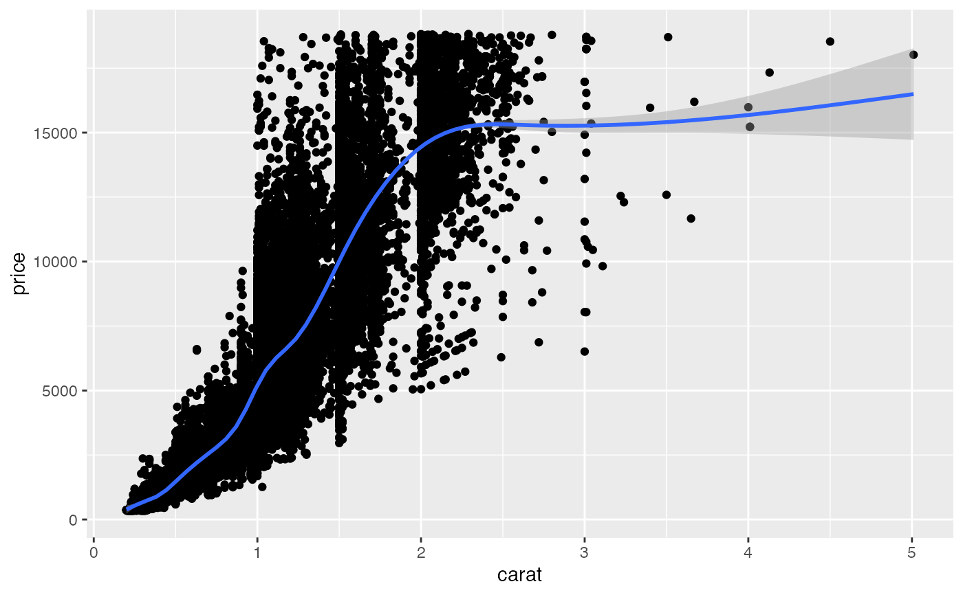
#>#> #> Call: #> lm(formula = mpg ~ well_knotted_spline(wt, 3), data = mtcars) #> #> Coefficients: #> (Intercept) well_knotted_spline(wt, 3)1 #> 32.13 -17.46 #> well_knotted_spline(wt, 3)2 well_knotted_spline(wt, 3)3 #> -17.82 -26.07 #> well_knotted_spline(wt, 3)4 #> -15.17 #># When insufficient unique values exist, less knots are used lm(mpg ~ well_knotted_spline(gear,3), data=mtcars)#>#> #> Call: #> lm(formula = mpg ~ well_knotted_spline(gear, 3), data = mtcars) #> #> Coefficients: #> (Intercept) well_knotted_spline(gear, 3)1 #> 16.1067 14.8746 #> well_knotted_spline(gear, 3)2 #> 0.9145 #>library(ggplot2) ggplot(diamonds, aes(carat, price)) + geom_point() + geom_smooth(method="lm", formula=y~well_knotted_spline(x,10))#>