Let’s look at the airway dataset as an example of a typical small-scale RNA-Seq experiment. In this experiment, four Airway Smooth Muscle (ASM) cell lines are treated with the asthma medication dexamethasone.

library(weitrix)
library(SummarizedExperiment)
library(EnsDb.Hsapiens.v86)
library(edgeR)
library(limma)
library(reshape2)
library(tidyverse)
library(airway)

set.seed(1234)

data("airway")
airway

## class: RangedSummarizedExperiment 
## dim: 64102 8 
## metadata(1): ''
## assays(1): counts
## rownames(64102): ENSG00000000003 ENSG00000000005 ... LRG_98 LRG_99
## rowData names(0):
## colnames(8): SRR1039508 SRR1039509 ... SRR1039520 SRR1039521
## colData names(9): SampleName cell ... Sample BioSample

Initial processing

Initial steps are the same as for a differential expression analysis.

counts <- assay(airway,"counts")

# Keep genes with an average of at least 1 read per sample
good <- rowMeans(counts) >= 1 
table(good)

## good
## FALSE  TRUE 
## 40931 23171

airway_cpm <- 
    DGEList(counts[good,]) %>%
    calcNormFactors() %>%
    cpm(log=TRUE, prior.count=1)

design <- model.matrix(~ dex + cell, data=colData(airway))

airway_elist <- vooma(airway_cpm, design=design, plot=TRUE)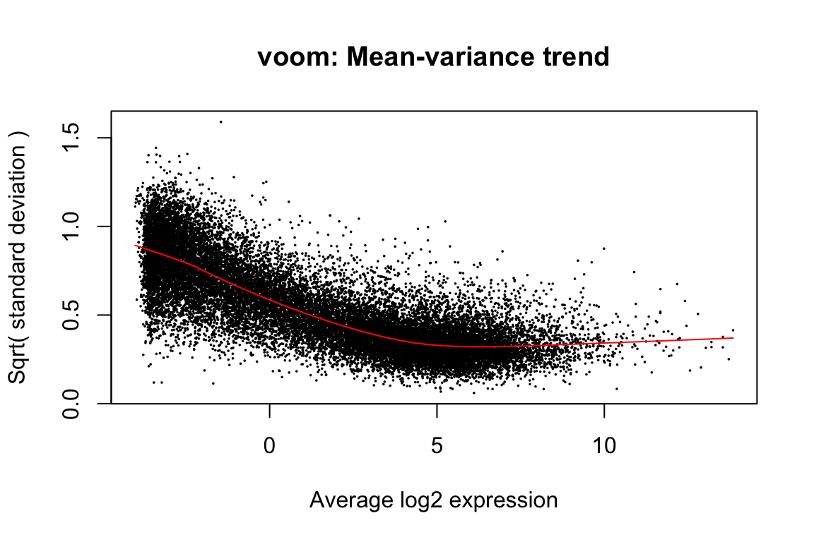

Some of these steps are optional and have marginal value:

vooma provides precision weights. One could instead choose a prior.count for cpm to produce a flat (or at least non-decreasing) mean-variance trend-line.
Using a design matrix with vooma may not provide much benefit, and if you want an analysis completely blinded to the experimental design it might be better to omit this.

There are many options here, so adjust to your taste!

Conversion to weitrix

airway_weitrix <- as_weitrix(airway_elist)

# Include row and column information
colData(airway_weitrix) <- colData(airway)
rowData(airway_weitrix) <- 
    mcols(genes(EnsDb.Hsapiens.v86))[rownames(airway_weitrix),c("gene_name","gene_biotype")]

airway_weitrix

## class: SummarizedExperiment 
## dim: 23171 8 
## metadata(1): weitrix
## assays(2): x weights
## rownames(23171): ENSG00000000003 ENSG00000000419 ... ENSG00000273487
##   ENSG00000273488
## rowData names(2): gene_name gene_biotype
## colnames(8): SRR1039508 SRR1039509 ... SRR1039520 SRR1039521
## colData names(9): SampleName cell ... Sample BioSample

Exploration

Find components of variation

This will find various numbers of components, from 1 to 6. In each case, the components discovered have varimax rotation applied to their gene loadings to aid interpretability. The result is a list of Components objects.

comp_seq <- weitrix_components_seq(airway_weitrix, p=6)
comp_seq

## [[1]]
## Components are: (Intercept), C1 
## $row :  23171 x 2 matrix
## $col :  8 x 2 matrix
## $R2  :  0.3990789 
## 
## [[2]]
## Components are: (Intercept), C1, C2 
## $row :  23171 x 3 matrix
## $col :  8 x 3 matrix
## $R2  :  0.6229488 
## 
## [[3]]
## Components are: (Intercept), C1, C2, C3 
## $row :  23171 x 4 matrix
## $col :  8 x 4 matrix
## $R2  :  0.790927 
## 
## [[4]]
## Components are: (Intercept), C1, C2, C3, C4 
## $row :  23171 x 5 matrix
## $col :  8 x 5 matrix
## $R2  :  0.8948288 
## 
## [[5]]
## Components are: (Intercept), C1, C2, C3, C4, C5 
## $row :  23171 x 6 matrix
## $col :  8 x 6 matrix
## $R2  :  0.9388779 
## 
## [[6]]
## Components are: (Intercept), C1, C2, C3, C4, C5, C6 
## $row :  23171 x 7 matrix
## $col :  8 x 7 matrix
## $R2  :  0.972438

rand_weitrix <- weitrix_randomize(airway_weitrix)
rand_comp <- weitrix_components(rand_weitrix, p=1)

components_seq_screeplot(comp_seq, rand_comp)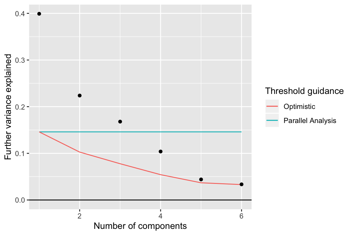

Examining components

Up to 4 components may be justified.

comp <- comp_seq[[4]]

comp$col[,-1] %>% melt(varnames=c("Run","component")) %>%
    left_join(as.data.frame(colData(airway)), by="Run") %>%
    ggplot(aes(y=cell, x=value, color=dex)) + 
    geom_vline(xintercept=0) + 
    geom_point(alpha=0.5, size=3) + 
    facet_grid(~ component) +
    labs(title="Sample scores for each component", x="Sample score", y="Cell line", color="Treatment")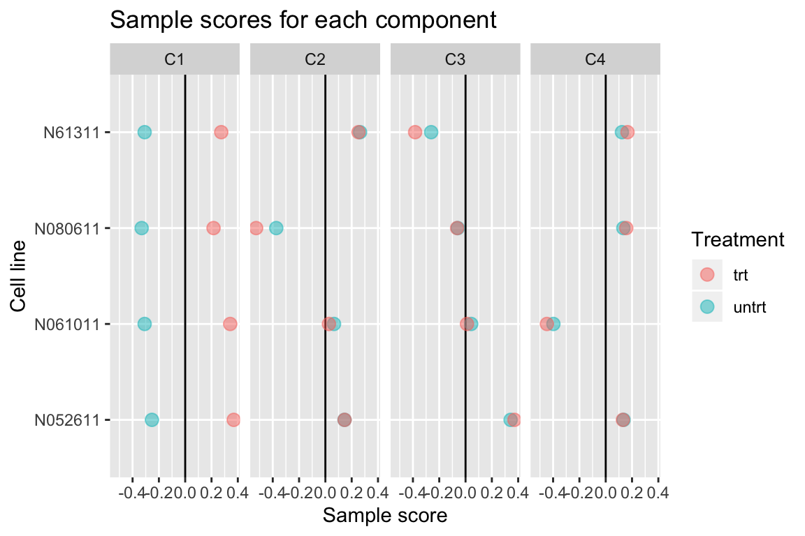

comp$row[,-1] %>% melt(varnames=c("name","component")) %>%
    ggplot(aes(x=comp$row[name,"(Intercept)"], y=value)) + 
    geom_point(cex=0.5, alpha=0.5) + 
    facet_wrap(~ component) +
    labs(title="Gene loadings for each component vs average log2 RPM", x="average log2 RPM", y="gene loading")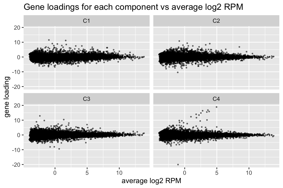

Without varimax rotation, components may be harder to interpret

If varimax rotation isn’t used, weitrix_components and weitrix_components_seq will produce a Principal Components Analysis, with components ordered from most to least variance explained.

Without varimax rotation the treatment effect is still mostly in the first component, but has also leaked a small amount into the other components.

comp_nonvarimax <- weitrix_components(airway_weitrix, p=4, use_varimax=FALSE)

comp_nonvarimax$col[,-1] %>% melt(varnames=c("Run","component")) %>%
    left_join(as.data.frame(colData(airway)), by="Run") %>%
    ggplot(aes(y=cell, x=value, color=dex)) + 
    geom_vline(xintercept=0) + 
    geom_point(alpha=0.5, size=3) + 
    facet_grid(~ component) +
    labs(title="Sample scores for each component, no varimax rotation", x="Sample score", y="Cell line", color="Treatment")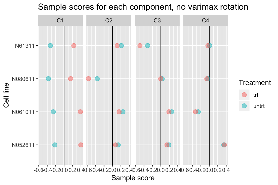

`col` can potentially be used as a design matrix with limma

If you are willing to place your trust in sparsity of effects, this may be a somewhat magical way of removing unwanted variation.
If you’re not sure of the experimental design, for example the exact timing of a time series or how evenly a drug treatment was applied, the extracted component might actually be more accurate.

Note that this ignores uncertainty about the col matrix itself.

This may be useful for hypothesis generation – finding some potentially interesting genes, while discounting noisy or lowly expressed genes – but don’t use it as proof of significance.

airway_elist <- weitrix_elist(airway_weitrix)

fit <- 
    lmFit(airway_elist, comp$col) %>% 
    eBayes()

fit$df.prior

## [1] 8.595638

fit$s2.prior

## [1] 1.076146

topTable(fit, "C1")

##                 gene_name   gene_biotype     logFC  AveExpr         t
## ENSG00000101347    SAMHD1 protein_coding  6.283933 8.134279  48.58913
## ENSG00000189221      MAOA protein_coding  5.482452 5.950311  36.06758
## ENSG00000178695    KCTD12 protein_coding -4.227635 6.450973 -32.96743
## ENSG00000139132      FGD4 protein_coding  3.652991 5.415156  31.41780
## ENSG00000120129     DUSP1 protein_coding  4.895673 6.643767  31.01784
## ENSG00000179094      PER1 protein_coding  5.204844 4.421867  30.98882
## ENSG00000124766      SOX4 protein_coding -4.084065 5.426691 -29.55701
## ENSG00000162692     VCAM1 protein_coding -6.134506 3.575005 -31.34264
## ENSG00000134243     SORT1 protein_coding  3.596138 7.568421  27.48157
## ENSG00000163884     KLF15 protein_coding  7.483922 3.248049  31.70319
##                      P.Value    adj.P.Val        B
## ENSG00000101347 9.185497e-15 2.128371e-10 23.17495
## ENSG00000189221 2.848140e-13 3.299712e-09 20.50857
## ENSG00000178695 8.000298e-13 4.714209e-09 19.72905
## ENSG00000139132 1.390192e-12 4.714209e-09 19.19450
## ENSG00000120129 1.610249e-12 4.714209e-09 19.10150
## ENSG00000179094 1.627624e-12 4.714209e-09 18.69549
## ENSG00000124766 2.799112e-12 7.022876e-09 18.54653
## ENSG00000162692 1.428917e-12 4.714209e-09 18.11379
## ENSG00000134243 6.439868e-12 1.243485e-08 17.84781
## ENSG00000163884 1.253204e-12 4.714209e-09 17.75410

all_top <- topTable(fit, "C1", n=Inf, sort.by="none")
plotMD(fit, "C1", status=all_top$adj.P.Val <= 0.01)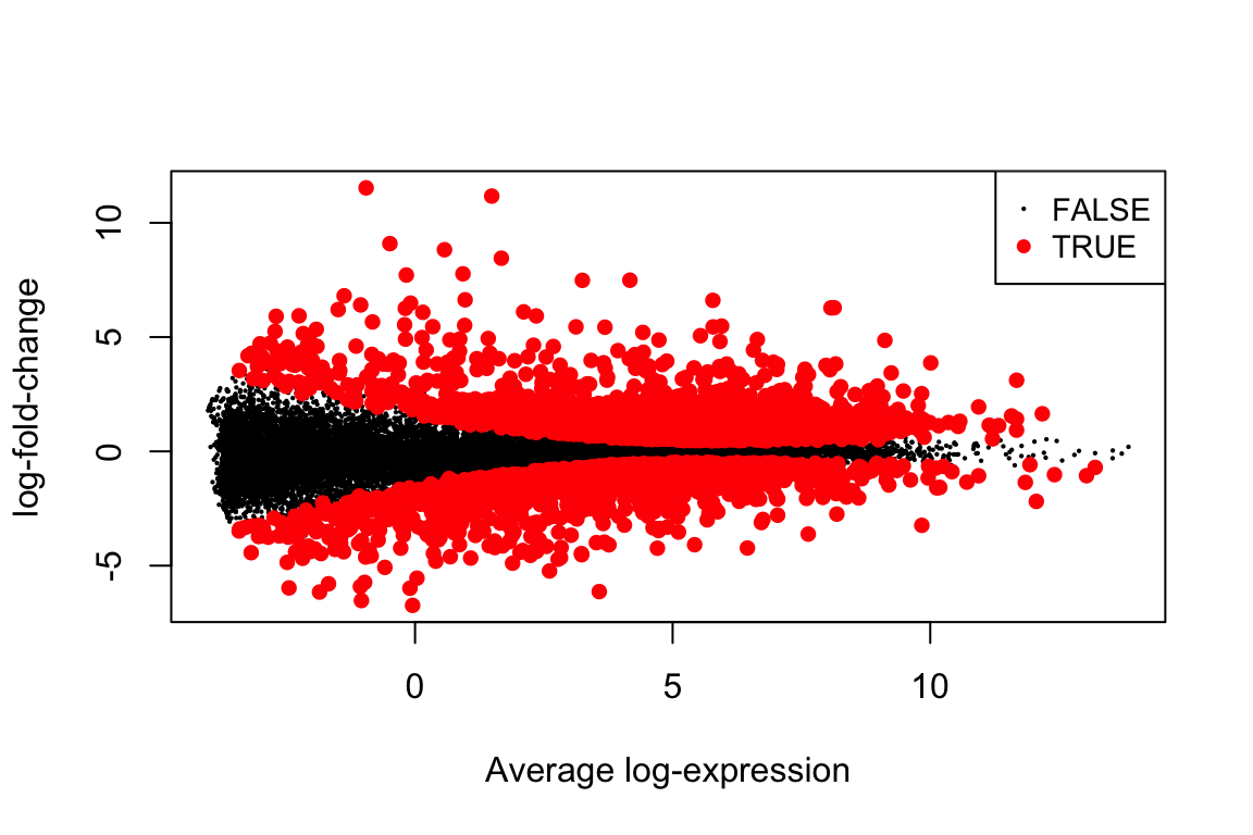

You might also consider using my topconfects package. This will find the largest confident effect sizes, while still correcting for multiple testing.

library(topconfects)
limma_confects(fit, "C1")

## $table
##  rank index confect effect    AveExpr    name            gene_name    
##   1   12120  6.665  11.528546 -0.9495193 ENSG00000179593 ALOX15B      
##   2    3272  6.608  11.169008  1.4890296 ENSG00000109906 ZBTB16       
##   3   11016  5.832   8.822691  0.5713077 ENSG00000171819 ANGPTL7      
##   4    9499  5.832   7.483922  3.2480486 ENSG00000163884 KLF15        
##   5    8175  5.744   7.488661  4.1705059 ENSG00000152583 SPARCL1      
##   6    2230  5.416   6.283933  8.1342789 ENSG00000101347 SAMHD1       
##   7    5156  5.375   8.450418  1.6752492 ENSG00000127954 STEAP4       
##   8   10420  5.189   7.767901  0.9298793 ENSG00000168309 FAM107A      
##   9   19752  4.935   9.090523 -0.4883206 ENSG00000250978 RP11-357D18.1
##  10    9220 -4.892  -6.134506  3.5750054 ENSG00000162692 VCAM1        
##  gene_biotype        
##  protein_coding      
##  protein_coding      
##  protein_coding      
##  protein_coding      
##  protein_coding      
##  protein_coding      
##  protein_coding      
##  protein_coding      
##  processed_transcript
##  protein_coding      
## ...
## 5534 of 23171 non-zero log2 fold change at FDR 0.05
## Prior df 8.6

RNA-Seq components, airway dataset, using cpm+vooma

Initial processing

Conversion to weitrix

Exploration

Find components of variation

Examining components

Without varimax rotation, components may be harder to interpret

`col` can potentially be used as a design matrix with limma

Contents

RNA-Seq components, airway dataset, using cpm+vooma

Initial processing

Conversion to weitrix

Exploration

Find components of variation

Examining components

Without varimax rotation, components may be harder to interpret

col can potentially be used as a design matrix with limma

Contents

`col` can potentially be used as a design matrix with limma