2. poly(A) tail length example
tail_length.Rmdpoly(A) tail length of transcripts can be measured using the PAT-Seq protocol. This protocol produces 3’-end focussed reads that include the poly(A) tail. We examine GSE83162. This is a time-series experiment in which two strains of yeast are released into synchronized cell cycling and observed through two cycles. Yeast are treated with \(\alpha\)-factor, which causes them to stop dividing in antici… pation of a chance to mate. When the \(\alpha\)-factor is washed away, they resume cycling.
Read files, extract experimental design from sample names
library(tidyverse)
library(reshape2)
library(SummarizedExperiment)
library(limma)
library(topconfects)
library(org.Sc.sgd.db)
library(weitrix)

tail <- system.file("GSE83162", "tail.csv.gz", package="weitrix") %>%
    read_csv() %>%
    column_to_rownames("Feature") %>%
    as.matrix()

tail_count <- system.file("GSE83162", "tail_count.csv.gz", package="weitrix") %>%
    read_csv() %>%
    column_to_rownames("Feature") %>%
    as.matrix()

samples <- data.frame(sample=I(colnames(tail))) %>%
    extract(sample, c("strain","time"), c("(.+)-(.+)"), remove=FALSE) %>%
    mutate(
        strain=factor(strain,unique(strain)),
        time=factor(time,unique(time)))
rownames(samples) <- colnames(tail)

samples
## sample strain time
## WT-tpre WT-tpre WT tpre
## WT-t0m WT-t0m WT t0m
## WT-t15m WT-t15m WT t15m
## WT-t30m WT-t30m WT t30m
## WT-t45m WT-t45m WT t45m
## WT-t60m WT-t60m WT t60m
## WT-t75m WT-t75m WT t75m
## WT-t90m WT-t90m WT t90m
## WT-t105m WT-t105m WT t105m
## WT-t120m WT-t120m WT t120m
## DeltaSet1-tpre DeltaSet1-tpre DeltaSet1 tpre
## DeltaSet1-t0m DeltaSet1-t0m DeltaSet1 t0m
## DeltaSet1-t15m DeltaSet1-t15m DeltaSet1 t15m
## DeltaSet1-t30m DeltaSet1-t30m DeltaSet1 t30m
## DeltaSet1-t45m DeltaSet1-t45m DeltaSet1 t45m
## DeltaSet1-t60m DeltaSet1-t60m DeltaSet1 t60m
## DeltaSet1-t75m DeltaSet1-t75m DeltaSet1 t75m
## DeltaSet1-t90m DeltaSet1-t90m DeltaSet1 t90m
## DeltaSet1-t105m DeltaSet1-t105m DeltaSet1 t105m
## DeltaSet1-t120m DeltaSet1-t120m DeltaSet1 t120m“tpre” is the cells in an unsynchronized state, other times are minutes after release into cycling.
The two strains are a wildtype and a strain with a mutated set1 gene.
Create weitrix object
From experience, noise scales with the length of the tail. Therefore to stabilize the variance we will be examing log2 of the tail length.
These tail lengths are each the average over many reads. We therefore weight each tail length by the number of reads. This is somewhat overoptimistic as there is biological noise that doesn’t go away with more reads, which we will correct for in the next step.
## good
## FALSE  TRUE
## 1657 4875Calibration
Our first step is to calibrate our weights. Our weights are overoptimistic for large numbers of reads, as there is a biological components of noise that does not go away with more reads.
Calibration requires a model explaining non-random effects. We provide a design matrix and a weighted linear model fit is found for each row. The lack of replicates makes life difficult, for simplicity here we will assume time and strain are independent.
design <- model.matrix(~ strain + time, data=colData(wei))The dispersion is then calculated for each row. A spline curve is fitted to the log dispersion. Weights in each row are then scaled so as to flatten this curve.
cal_design <- weitrix_calibrate_trend(wei, design, ~splines::ns(log2(total_reads),3))Examining the effect of calibration
Let’s unpack what happens in that weitrix_calibrate_trend step.
rowData(cal_design)$dispersion_unweighted <- weitrix_dispersions(weitrix_x(wei), design)Consider first the dispersion if weights were uniform. Missing data is weighted 0, all other weights are 1.
rowData(cal_design) %>% as.data.frame() %>%
    ggplot(aes(x=total_reads, y=dispersion_unweighted)) + geom_point(size=0.1) +
    scale_x_log10() + scale_y_log10() +
    labs(title="Dispersion if uniform weights used (log scales)")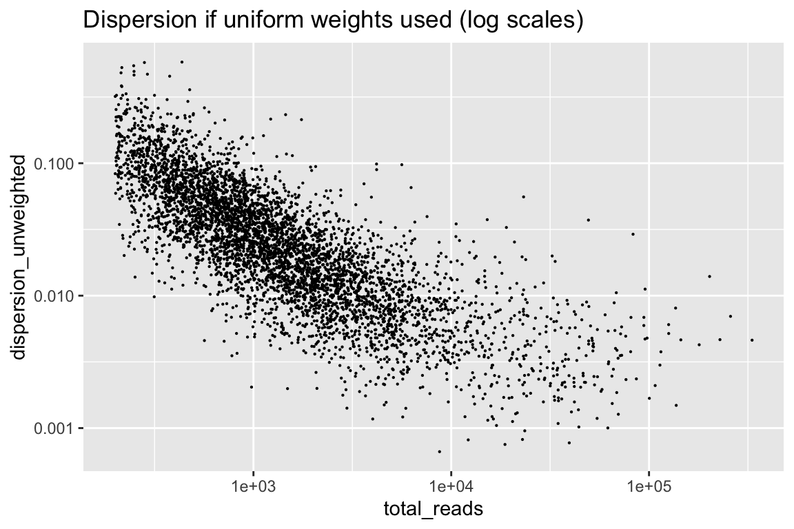
There is information from the number of reads that we can remove.
Here are the dispersions using read-counts as weights.
rowData(cal_design) %>% as.data.frame() %>%
    ggplot(aes(x=total_reads, y=dispersion_before)) + geom_point(size=0.1) +
    geom_line(aes(y=dispersion_trend), color="red") +
    scale_x_log10() + scale_y_log10() +
    labs(title="Dispersion with read-counts as weights (log scales)")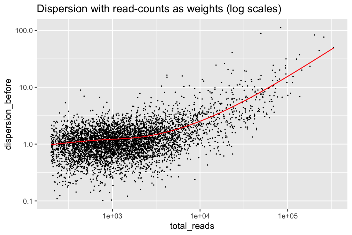
In general it is improved, but now we have the opposite problem. There is a component of noise that does not go away with more and more reads. The red line is a trend fitted to this, which weitrix_calibrate_trend divides out of the weights.
Finally, here are the dispersion from the calibrated weitrix.
rowData(cal_design) %>% as.data.frame() %>%
    ggplot(aes(x=total_reads, y=dispersion_after)) + geom_point(size=0.1) +
    scale_x_log10() + scale_y_log10() +
    labs(title="Dispersion with read-count weights / trend-based calibration\n(log scales)")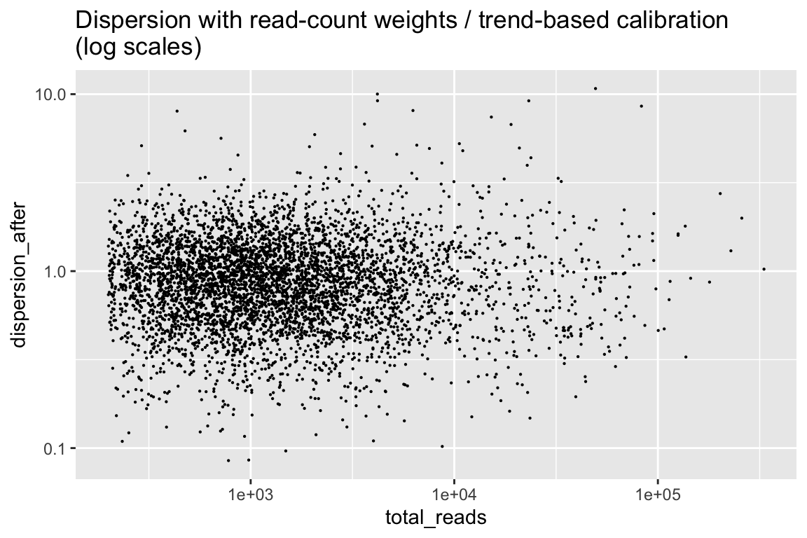
This is reasonably close to uniform, with no trend from the number of reads. limma can now estimate the variability of dispersions between genes, and apply its Emprical-Bayes squeezed dispersion based testing.
Testing
We are now ready to test things. We feed our calibrated weitrix to limma.
fit_cal_design <- cal_design %>%
    weitrix_elist() %>%
    lmFit(design)

ebayes_fit <- eBayes(fit_cal_design)
result_signif <- topTable(ebayes_fit, "strainDeltaSet1", n=Inf)

result_signif %>%
    dplyr::select(gene,diff_log2_tail=logFC,ave_log2_tail=AveExpr,
        adj.P.Val,total_reads) %>%
    head(20)
## gene diff_log2_tail ave_log2_tail adj.P.Val total_reads
## YDR170W-A <NA> -0.3317487 4.679897 3.440790e-06 4832
## YJR027W/YJR026W <NA> -0.2564543 4.271790 2.287980e-05 6577
## YAR009C <NA> -0.4673765 3.931000 2.287980e-05 1866
## YIL015W BAR1 -0.3653600 4.893617 6.233632e-05 3898
## YPL257W-B/YPL257W-A <NA> -0.2558543 4.209088 1.151177e-04 5729
## YML045W/YML045W-A <NA> -0.2406881 4.354082 1.953731e-04 4553
## YLR157C-B/YLR157C-A <NA> -0.2224134 4.200638 3.860716e-04 5519
## YGR027W-B/YGR027W-A <NA> -0.2093877 4.206404 4.750243e-04 5685
## YLR035C-A <NA> -0.3804618 3.918629 5.945463e-04 1374
## YPR137C-B/YPR137C-A <NA> -0.2105818 4.257820 6.441298e-04 7287
## YER138C/YER137C-A <NA> -0.2053578 4.187405 7.537499e-04 5652
## YML039W/YML040W <NA> -0.2343804 4.213771 7.928725e-04 5851
## YMR045C/YMR046C <NA> -0.2087868 4.266254 8.387704e-04 4579
## YJR029W/YJR028W <NA> -0.2062738 4.254686 1.128685e-03 5979
## YNL284C-B/YNL284C-A <NA> -0.1899551 4.370570 1.157811e-03 4830
## YPL217C BMS1 -0.3051718 4.086526 1.254310e-03 2071
## YPR158C-D/YPR158C-C <NA> -0.1975358 4.227524 1.254310e-03 5381
## YIL053W GPP1 -0.1463690 4.760486 1.480738e-03 25996
## YOR192C-B/YOR192C-A <NA> -0.4356656 4.397721 1.480738e-03 864
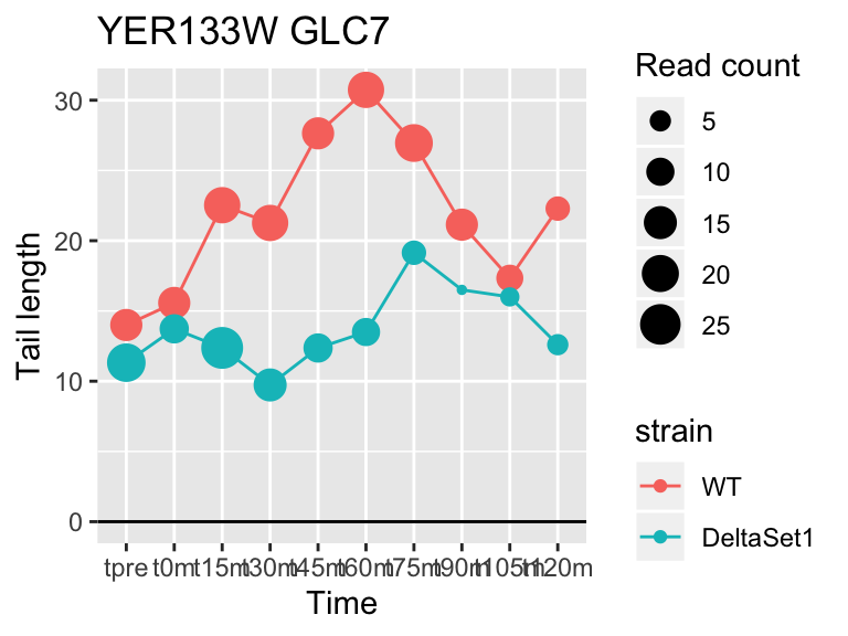
## YER133W GLC7 -0.7326781 4.084170 7.537499e-04 264My package topconfects can be used to find top confident differential tail length. Rather than picking “most significant” genes, it will highlight genes with a large effect size.
result_confects <- limma_confects(
    fit_cal_design, "strainDeltaSet1", full=TRUE, fdr=0.05)

result_confects$table %>%
    dplyr::select(gene,diff_log2_tail=effect,confect,total_reads) %>%
    head(20)
## gene diff_log2_tail confect total_reads
## YAR009C <NA> -0.4673765 -0.157 1866
## YDR170W-A <NA> -0.3317487 -0.151 4832
## YER133W GLC7 -0.7326781 -0.151 264
## YIL015W BAR1 -0.3653600 -0.131 3898
## YJR027W/YJR026W <NA> -0.2564543 -0.107 6577
## YLR035C-A <NA> -0.3804618 -0.102 1374
## YCR014C POL4 -0.4968279 -0.098 606
## YPL257W-B/YPL257W-A <NA> -0.2558543 -0.094 5729
## YOR192C-B/YOR192C-A <NA> -0.4356656 -0.094 864
## YML045W/YML045W-A <NA> -0.2406881 -0.085 4553
## YPL217C BMS1 -0.3051718 -0.074 2071
## YLR157C-B/YLR157C-A <NA> -0.2224134 -0.074 5519
## YGR027W-B/YGR027W-A <NA> -0.2093877 -0.068 5685
## YML039W/YML040W <NA> -0.2343804 -0.068 5851
## YDR476C <NA> -0.3794150 -0.067 4196
## YPR137C-B/YPR137C-A <NA> -0.2105818 -0.067 7287
## YER138C/YER137C-A <NA> -0.2053578 -0.063 5652
## YMR045C/YMR046C <NA> -0.2087868 -0.063 4579
## YJR029W/YJR028W <NA> -0.2062738 -0.060 5979
## YMR238W DFG5 -0.2478286 -0.060 2502## 80 genes significantly non-zero at FDR 0.05This lists the largest confident log2 fold changes in poly(A) tail length. The confect column is an inner confidence bound on the difference in log2 tail length, adjusted for multiple testing.
We discover some genes with less total reads, but large change in tail length.
Note that due to PCR amplification slippage and limited read length, the observed log2 poly(A) tail lengths may be an underestimate. However as all samples have been prepared in the same way, observed differences should indicate the existence of true differences.
Examine individual genes
Having discovered genes with differential tail length, let’s look at some genes in detail.
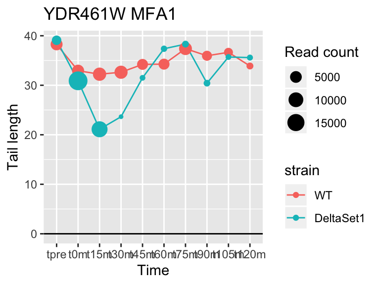
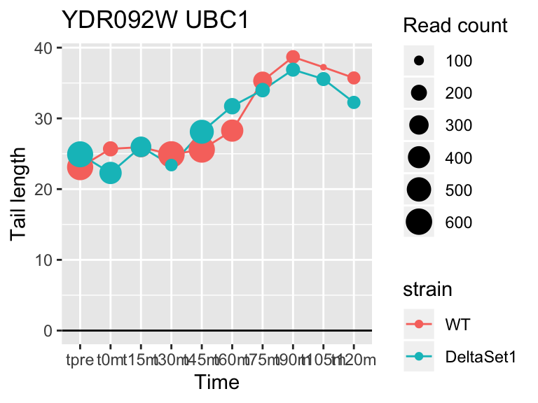
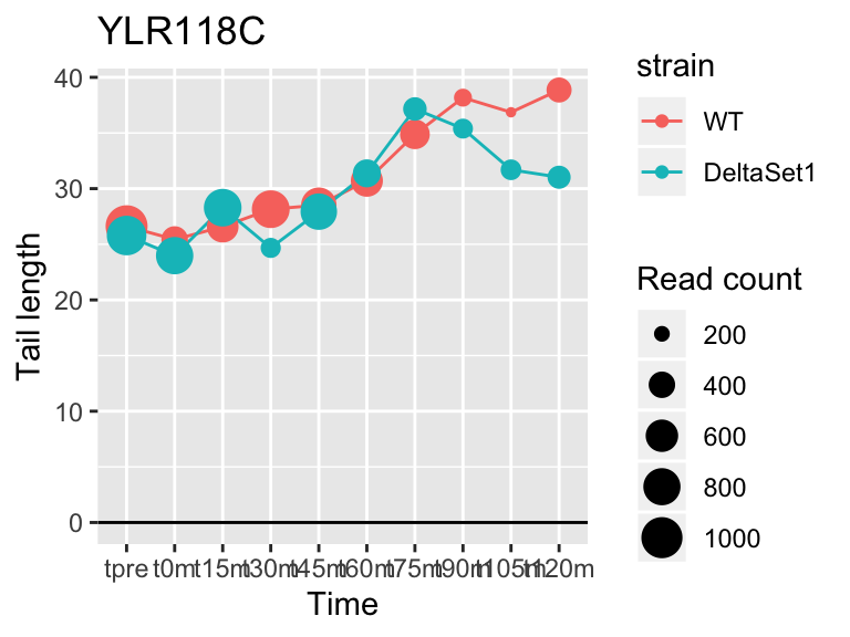
view_gene <- function(id, title="") {
ggplot(samples, aes(x=time,color=strain,group=strain, y=tail[id,])) +
geom_hline(yintercept=0) +
geom_line() +
geom_point(aes(size=tail_count[id,])) +
labs(x="Time", y="Tail length", size="Read count", title=paste(id,title))
}
# Top "significant" genes
view_gene("YDR170W-A")
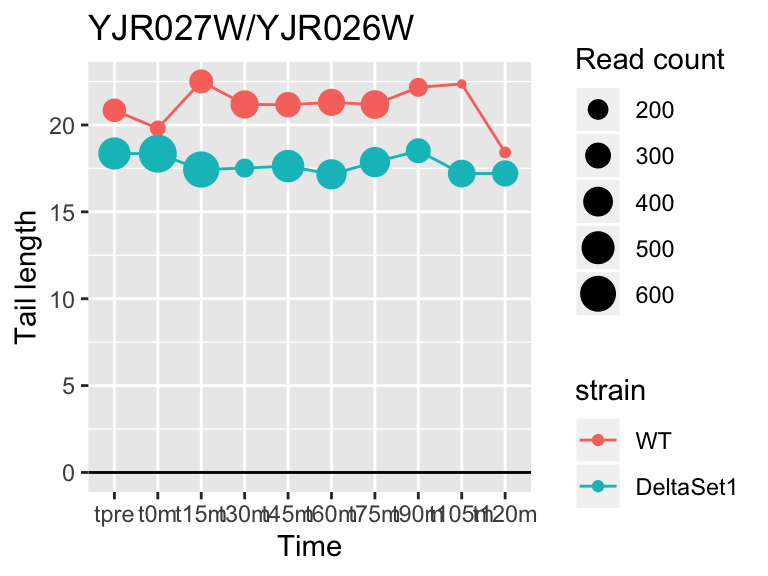
view_gene("YJR027W/YJR026W")
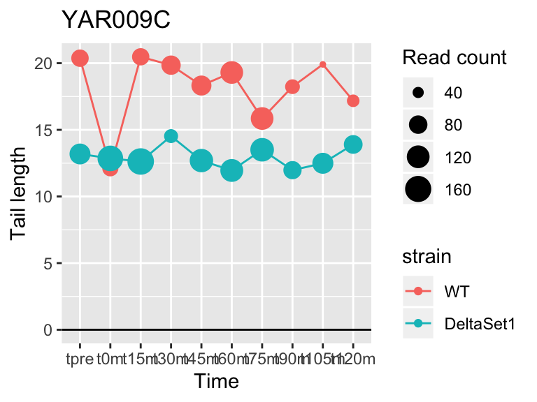
view_gene("YAR009C")
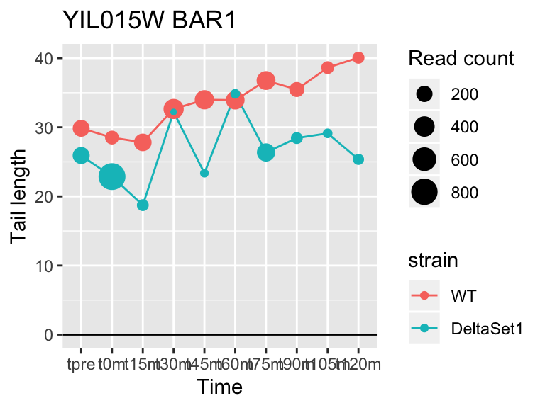
view_gene("YIL015W","BAR1")
# topconfects has highlighted some genes with lower total reads
view_gene("YER133W","GLC7")
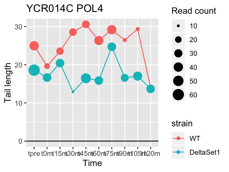
view_gene("YCR014C","POL4")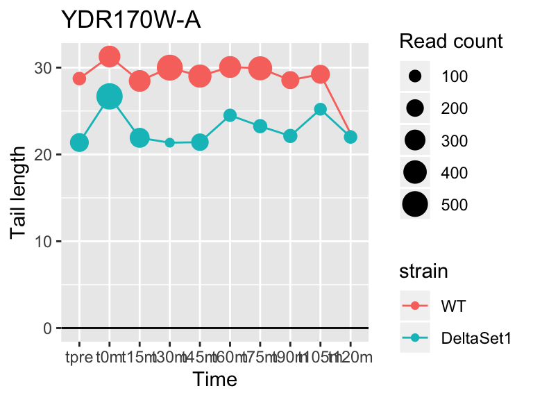

Exploratory analysis
We can also look for components of variation.
comp_seq <- weitrix_components_seq(wei, p=10)components_seq_screeplot(comp_seq)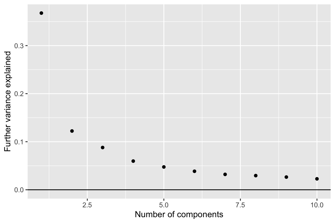
Looking at three components shows some of the major trends in this data-set.
comp <- comp_seq[[3]]

comp$col[,-1] %>% melt(varnames=c("sample","component")) %>%
    left_join(samples,by="sample") %>%
    ggplot(aes(x=time, y=value, color=strain, group=strain)) +
    geom_hline(yintercept=0) +
    geom_line() +
    geom_point(alpha=0.75, size=3) +
    facet_grid(component ~ .) +
    labs(title="Sample scores for each component", y="Sample score", x="Time", color="Strain")
## Warning: Column `sample` joining factor and character vector, coercing into
## character vector## Warning: Column `sample` has different attributes on LHS and RHS of join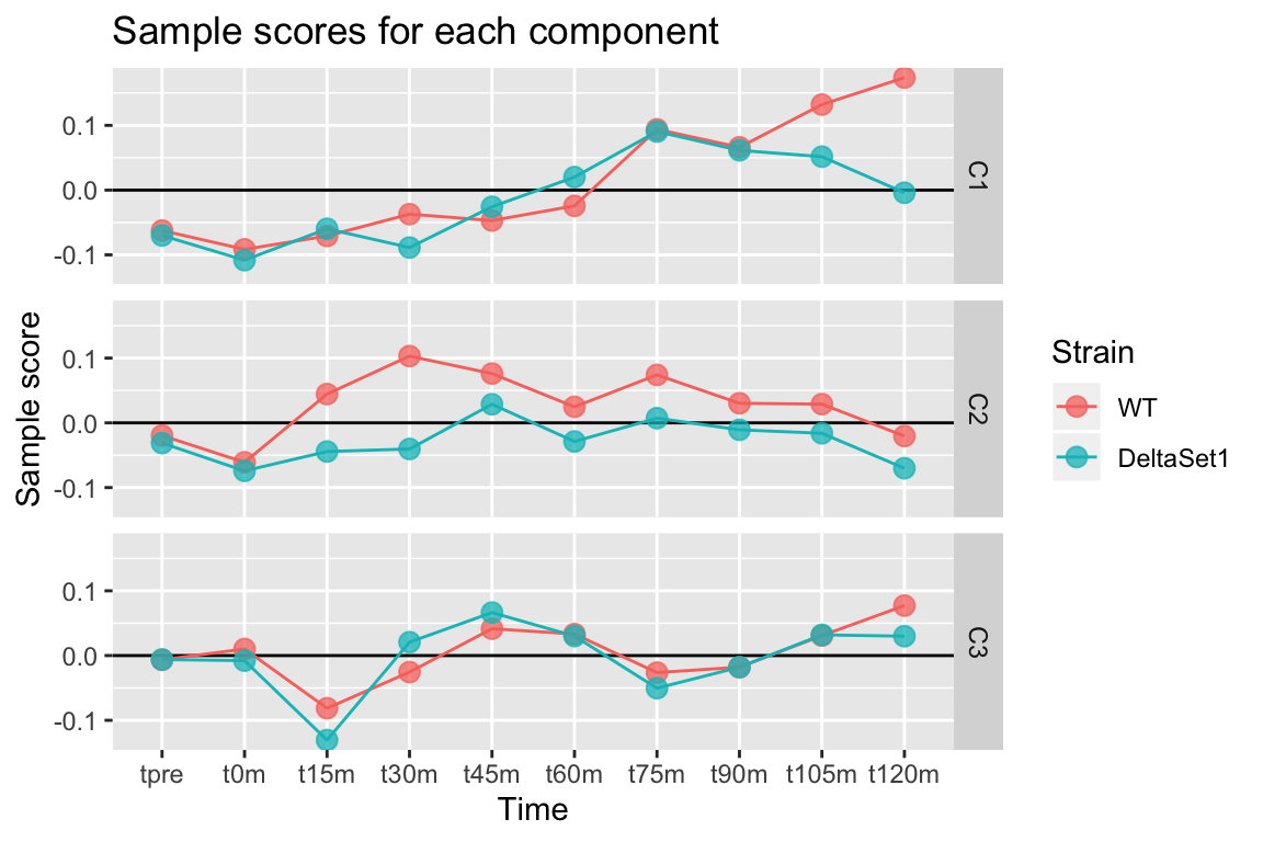
We observe:
- C1 - A gradual lengthening of tails after release into cell cycling. (The reason for the divergence between strains at the end is unclear.)
- C2 - A lengthening of poly(A) tails in the set1 mutant.
- C3 - Variation in poly(A) tail length with the cell cycle.
The log2 tail lengths are approximated by comp$row %*% t(comp$col) where comp$col is an \(n_\text{sample} \times (p+1)\) matrix of scores (shown above), and comp$row is an \(n_\text{gene} \times (p+1)\) matrix of gene loadings, which we will now examine. (The \(+1\) is the intercept “component”, allowing each gene to have a different baseline tail length.)
cal_comp <- weitrix_calibrate_trend(wei, comp, ~splines::ns(log2(total_reads),3))
fit_comp <- cal_comp %>%
    weitrix_elist() %>%
    lmFit(comp$col)
Treat these results with caution. Confindence bounds take into account uncertainty in the loadings but not in the scores! What follows is best regarded as exploratory rather than a final result.
Gene loadings for C1: gradual lengthing over time
result_C1 <- limma_confects(fit_comp, "C1")## gene loading confect total_reads
## YBL016W FUS3 3.863779 2.210 6287
## YOR096W RPS7A 3.284584 2.210 72660
## YDR092W UBC13 3.294252 1.863 6171
## YLR118C <NA> 2.670593 1.759 10599
## YDL185W VMA1 2.498601 1.658 22258
## YJL136C RPS21B 2.217832 1.544 179361
## YLR314C CDC3 2.167261 1.531 38826
## YGR090W UTP22 2.550122 1.505 6535
## YJL041W NSP1 2.445628 1.467 5463
## YMR142C RPL13B 2.121719 1.462 62128## 1137 genes significantly non-zero at FDR 0.05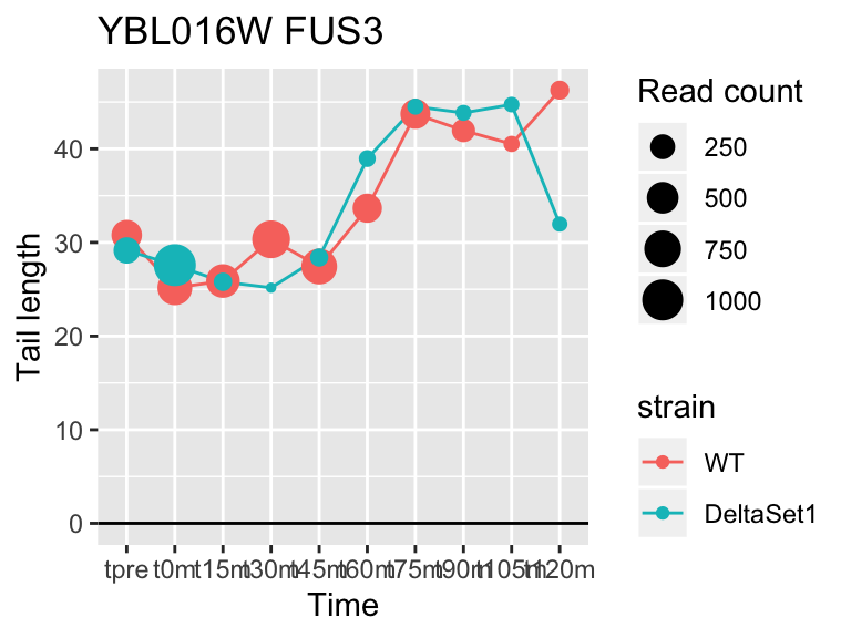
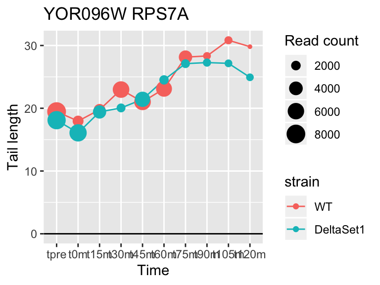
FUS3 is involved in yeast mating. We see here a poly(A) tail signature of yeast realizing there are not actually any \(\alpha\) cells around to mate with.
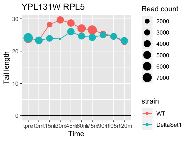
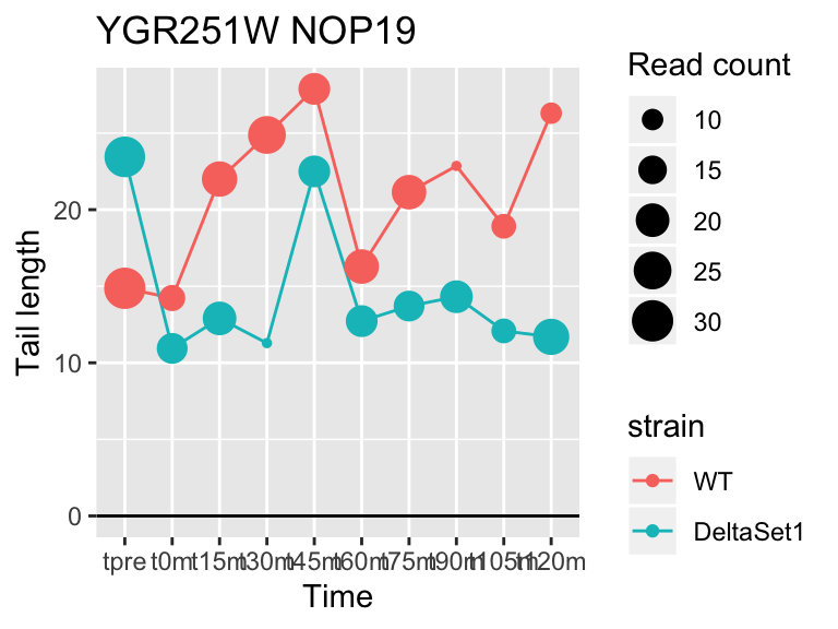
Gene loadings for C2: longer tails in set1 mutant
result_C2 <- limma_confects(fit_comp, "C2")## gene loading confect total_reads
## YDR476C <NA> 5.962351 2.794 4196
## YPL131W RPL5 2.093424 1.218 81051
## YCR014C POL4 5.844536 1.096 606
## YGR251W NOP19 6.503427 1.041 359
## YNL178W RPS3 1.922230 1.041 46065
## YIL015W BAR1 2.759544 0.996 3898
## YLR340W RPP0 1.967901 0.988 25545
## YLR035C-A <NA> 4.144392 0.943 1374
## YDL130W RPP1B 1.853441 0.883 68331
## YDR450W RPS18A 1.824185 0.878 30283## 409 genes significantly non-zero at FDR 0.05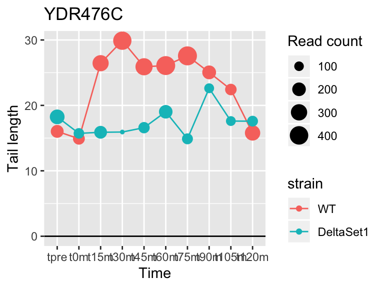
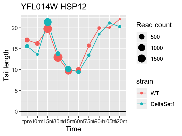
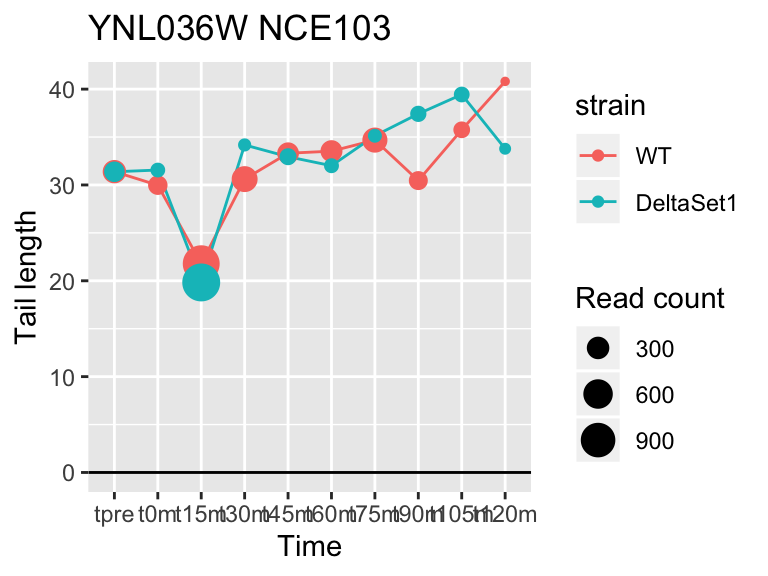
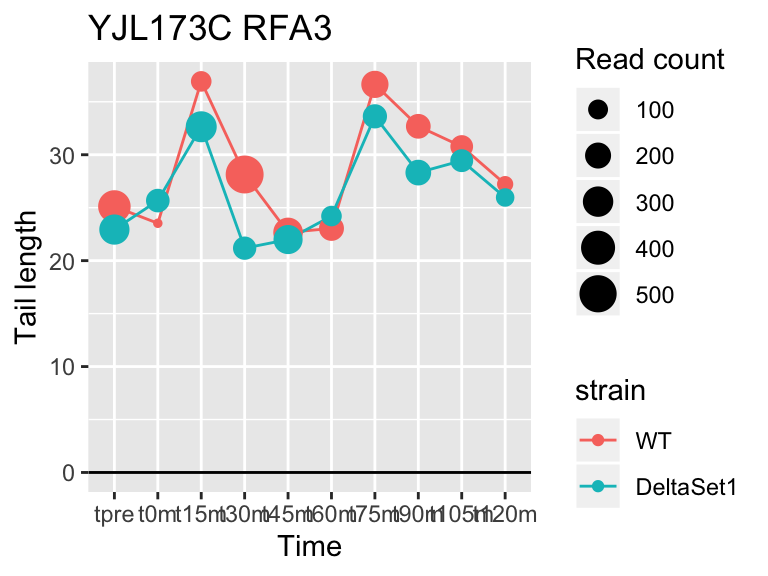
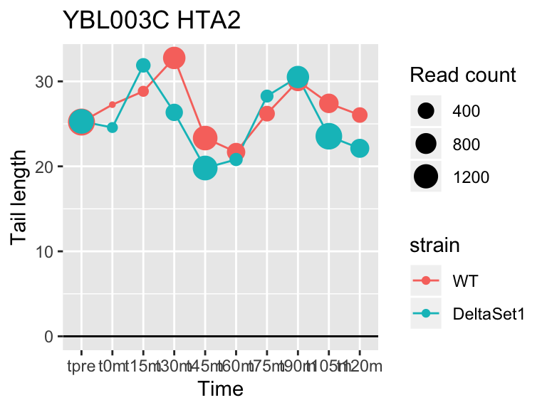
Gene loadings for C3: cell-cycle associated changes
result_C3 <- limma_confects(fit_comp, "C3")Given the mixture of signs for effects in C3, different genes are longer in different stages of the cell cycle. We see many genes to do with replication, and also Mating Factor A.
##             gene   loading confect total_reads
## YFL014W    HSP12 -5.624068  -2.633        9509
## YNL036W   NCE103  4.452372   2.633        5712
## YJL173C     RFA3 -3.780392  -1.908        3963
## YBL003C     HTA2 -4.415526  -1.908       13473
## YDR097C     MSH6 -5.051116  -1.806         996
## YBR009C     HHF1 -4.460064  -1.795       33533
## YEL011W     GLC3  4.417161   1.795         710
## YDR461W     MFA1  3.694856   1.604       83042
## YLR342W-A   <NA> -3.323401  -1.604       12356
## YBR092C     PHO3  3.759809   1.497        8441
## 157 genes significantly non-zero at FDR 0.05