RNA-Seq components, airway dataset, using cpm+weitrix_calibrate_trend
airway_calibrate.RmdLet’s look at the airway dataset as an example of a typical small-scale RNA-Seq experiment. In this experiment, four Airway Smooth Muscle (ASM) cell lines are treated with the asthma medication dexamethasone.
library(weitrix)
library(SummarizedExperiment)
library(EnsDb.Hsapiens.v86)
library(edgeR)
library(limma)
library(reshape2)
library(tidyverse)
library(airway)

set.seed(1234)data("airway")
airway## class: RangedSummarizedExperiment
## dim: 64102 8
## metadata(1): ''
## assays(1): counts
## rownames(64102): ENSG00000000003 ENSG00000000005 ... LRG_98 LRG_99
## rowData names(0):
## colnames(8): SRR1039508 SRR1039509 ... SRR1039520 SRR1039521
## colData names(9): SampleName cell ... Sample BioSampleInitial processing
Initial steps are the same as for a differential expression analysis.
counts <- assay(airway,"counts")

# Keep genes with an average of at least 1 read per sample
good <- rowMeans(counts) >= 1
table(good)
## good
## FALSE TRUE
## 40931 23171airway_lcpm <-
DGEList(counts[good,]) %>%
calcNormFactors() %>%
cpm(log=TRUE, prior.count=1)Conversion to weitrix
airway_weitrix <- as_weitrix(airway_lcpm)

# Include row and column information
colData(airway_weitrix) <- colData(airway)
rowData(airway_weitrix) <-
    mcols(genes(EnsDb.Hsapiens.v86))[rownames(airway_weitrix),c("gene_name","gene_biotype")]

rowData(airway_weitrix)$mean_lcpm <- rowMeans(airway_lcpm)

airway_weitrix
## class: SummarizedExperiment
## dim: 23171 8
## metadata(1): weitrix
## assays(2): x weights
## rownames(23171): ENSG00000000003 ENSG00000000419 ... ENSG00000273487
## ENSG00000273488
## rowData names(3): gene_name gene_biotype mean_lcpm
## colnames(8): SRR1039508 SRR1039509 ... SRR1039520 SRR1039521
## colData names(9): SampleName cell ... Sample BioSampleExploration
Find components of variation
This will find various numbers of components, from 1 to 6. In each case, the components discovered have varimax rotation applied to their gene loadings to aid interpretability. The result is a list of Components objects.
comp_seq <- weitrix_components_seq(airway_weitrix, p=6)
comp_seq
## [[1]]
## Components are: (Intercept), C1
## $row : 23171 x 2 matrix
## $col : 8 x 2 matrix
## $R2 : 0.2584425
##
## [[2]]
## Components are: (Intercept), C1, C2
## $row : 23171 x 3 matrix
## $col : 8 x 3 matrix
## $R2 : 0.4698357
##
## [[3]]
## Components are: (Intercept), C1, C2, C3
## $row : 23171 x 4 matrix
## $col : 8 x 4 matrix
## $R2 : 0.6423717
##
## [[4]]
## Components are: (Intercept), C1, C2, C3, C4
## $row : 23171 x 5 matrix
## $col : 8 x 5 matrix
## $R2 : 0.7915268
##
## [[5]]
## Components are: (Intercept), C1, C2, C3, C4, C5
## $row : 23171 x 6 matrix
## $col : 8 x 6 matrix
## $R2 : 0.866735
##
## [[6]]
## Components are: (Intercept), C1, C2, C3, C4, C5, C6
## $row : 23171 x 7 matrix
## $col : 8 x 7 matrix
## $R2 : 0.9355531rand_weitrix <- weitrix_randomize(airway_weitrix)
rand_comp <- weitrix_components(rand_weitrix, p=1)
components_seq_screeplot(comp_seq, rand_comp)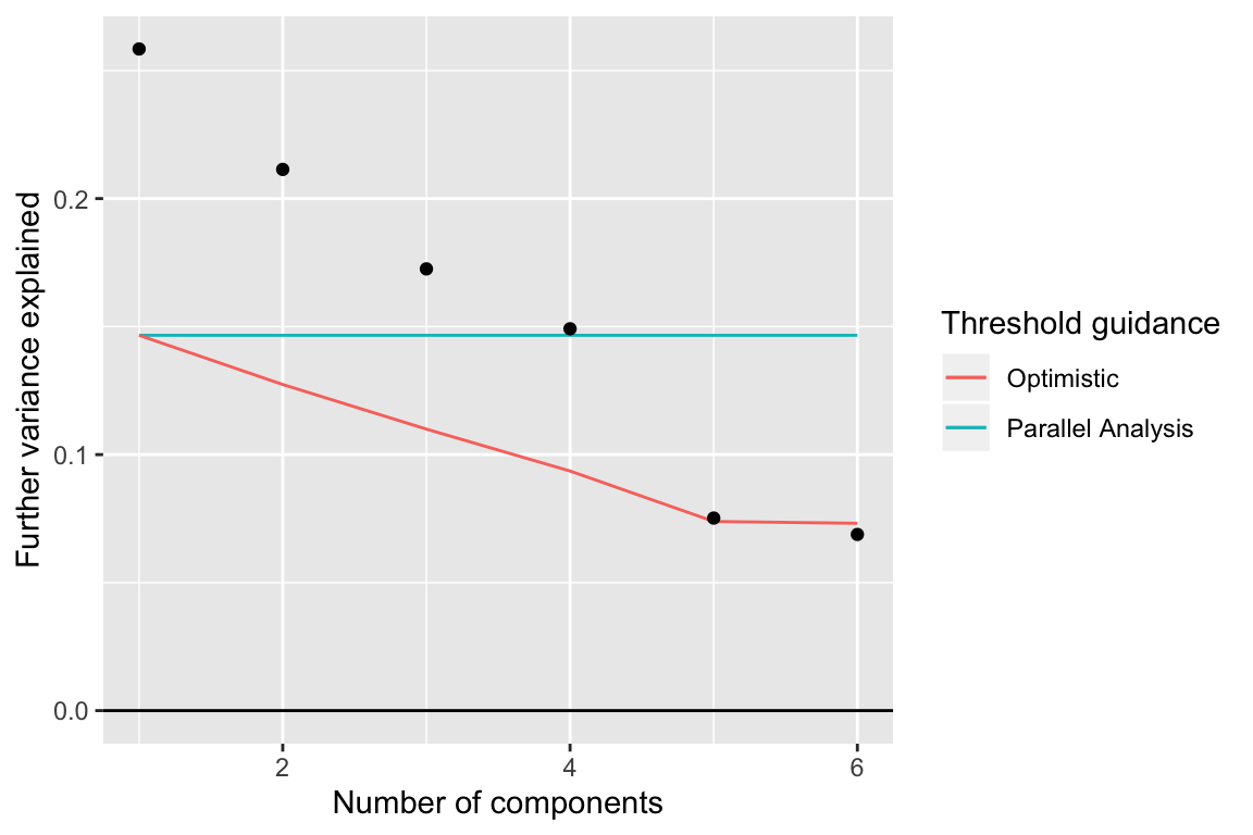
Examining components
Up to 4 components may be justified.
comp <- comp_seq[[4]]

comp$col[,-1] %>% melt(varnames=c("Run","component")) %>%
    left_join(as.data.frame(colData(airway)), by="Run") %>%
    ggplot(aes(y=cell, x=value, color=dex)) +
    geom_vline(xintercept=0) +
    geom_point(alpha=0.5, size=3) +
    facet_grid(~ component) +
    labs(title="Sample scores for each component", x="Sample score", y="Cell line", color="Treatment")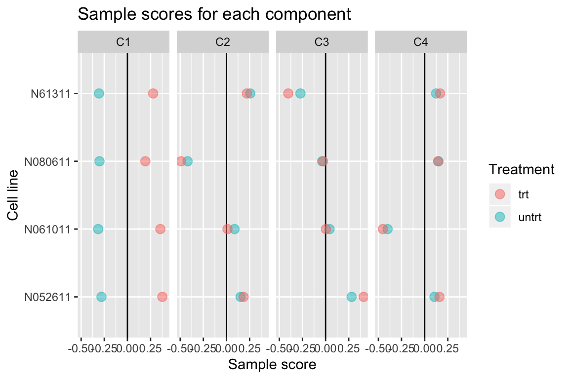
comp$row[,-1] %>% melt(varnames=c("name","component")) %>%
    ggplot(aes(x=comp$row[name,"(Intercept)"], y=value)) +
    geom_point(cex=0.5, alpha=0.5) +
    facet_wrap(~ component) +
    labs(title="Gene loadings for each component vs average log2 RPM", x="average log2 RPM", y="gene loading")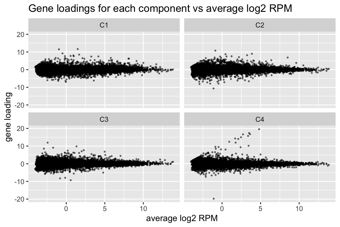
Without varimax rotation, components may be harder to interpret
If varimax rotation isn’t used, weitrix_components and weitrix_components_seq will produce a Principal Components Analysis, with components ordered from most to least variance explained.
Without varimax rotation the treatment effect is still mostly in the first component, but has also leaked a small amount into the other components.
comp_nonvarimax <- weitrix_components(airway_weitrix, p=4, use_varimax=FALSE)

comp_nonvarimax$col[,-1] %>% melt(varnames=c("Run","component")) %>%
    left_join(as.data.frame(colData(airway)), by="Run") %>%
    ggplot(aes(y=cell, x=value, color=dex)) +
    geom_vline(xintercept=0) +
    geom_point(alpha=0.5, size=3) +
    facet_grid(~ component) +
    labs(title="Sample scores for each component, no varimax rotation", x="Sample score", y="Cell line", color="Treatment")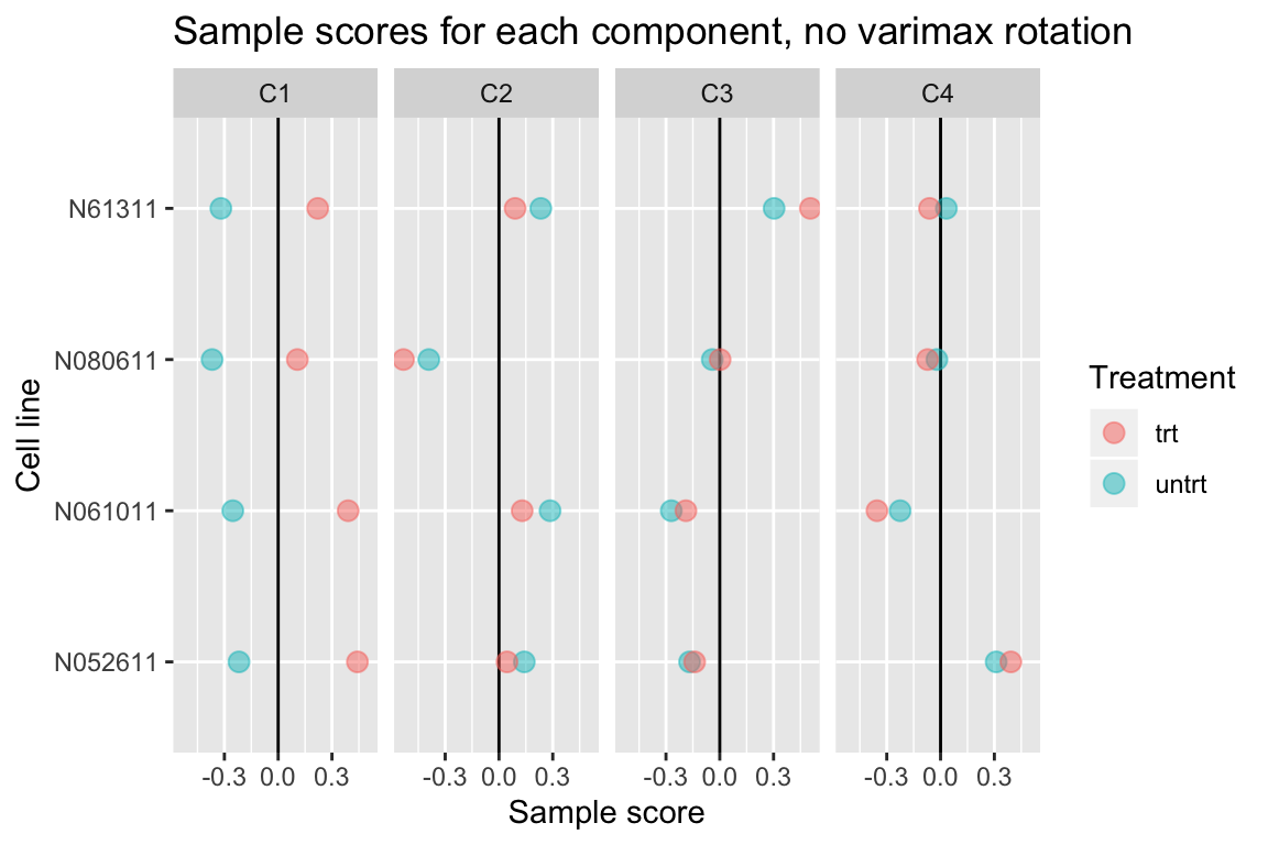
col can potentially be used as a design matrix with limma
If you are willing to place your trust in sparsity of effects, this may be a somewhat magical way of removing unwanted variation.
If you’re not sure of the experimental design, for example the exact timing of a time series or how evenly a drug treatment was applied, the extracted component might actually be more accurate.
Note that this ignores uncertainty about the col matrix itself.
This may be useful for hypothesis generation – finding some potentially interesting genes, while discounting noisy or lowly expressed genes – but don’t use it as proof of significance.
airway_cal <- weitrix_calibrate_trend(airway_weitrix, comp, ~splines::ns(mean_lcpm,3))

rowData(airway_cal) %>% as.data.frame() %>%
    ggplot(aes(x=mean_lcpm)) +
    geom_point(aes(y=dispersion_before^0.25), size=0.1) +
    geom_point(aes(y=dispersion_trend^0.25), size=0.1, color="red") +
    labs(x="Mean log2 RPM", y="sqrt( Standard deviation )")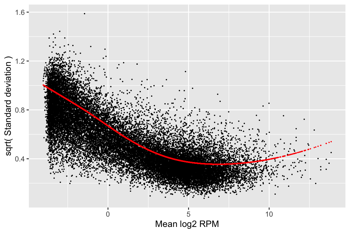
airway_elist <- weitrix_elist(airway_cal)

fit <-
    lmFit(airway_elist, comp$col) %>%
    eBayes()

fit$df.prior
## [1] 7.126632## [1] 0.6655365topTable(fit, "C1")## gene_name gene_biotype mean_lcpm dispersion_before
## ENSG00000101347 SAMHD1 protein_coding 8.134279 0.003891762
## ENSG00000179094 PER1 protein_coding 4.421867 0.001574842
## ENSG00000178695 KCTD12 protein_coding 6.450973 0.004614438
## ENSG00000124766 SOX4 protein_coding 5.426691 0.004098745
## ENSG00000163884 KLF15 protein_coding 3.248049 0.026366143
## ENSG00000096060 FKBP5 protein_coding 5.780916 0.062948554
## ENSG00000162692 VCAM1 protein_coding 3.575005 0.017149286
## ENSG00000138316 ADAMTS14 protein_coding 4.704289 0.005960254
## ENSG00000189221 MAOA protein_coding 5.950311 0.044149345
## ENSG00000139132 FGD4 protein_coding 5.415156 0.005093694
## dispersion_trend dispersion_after logFC AveExpr t
## ENSG00000101347 0.01721555 0.22606085 6.255818 8.134279 56.17414
## ENSG00000179094 0.02237273 0.07039114 5.231899 4.421867 43.10960
## ENSG00000178695 0.01604936 0.28751540 -4.201354 6.450973 -38.42477
## ENSG00000124766 0.01780661 0.23018107 -4.053501 5.426691 -35.74850
## ENSG00000163884 0.03478772 0.75791514 7.404889 3.248049 41.11476
## ENSG00000096060 0.01694075 3.71580756 6.637774 5.780916 35.09532
## ENSG00000162692 0.03020135 0.56783174 -6.192439 3.575005 -38.49876
## ENSG00000138316 0.02070066 0.28792583 -4.254018 4.704289 -34.25394
## ENSG00000189221 0.01662975 2.65484115 5.471656 5.950311 32.65172
## ENSG00000139132 0.01784014 0.28551866 3.654105 5.415156 31.71501
## P.Value adj.P.Val B
## ENSG00000101347 5.703137e-14 1.321474e-09 20.92604
## ENSG00000179094 8.237520e-13 9.543579e-09 18.77160
## ENSG00000178695 2.623751e-12 1.215899e-08 18.38667
## ENSG00000124766 5.423673e-12 2.094532e-08 17.70294
## ENSG00000163884 1.327630e-12 1.025417e-08 17.61658
## ENSG00000096060 6.528277e-12 2.160953e-08 17.59993
## ENSG00000162692 2.573447e-12 1.215899e-08 17.50448
## ENSG00000138316 8.331085e-12 2.412995e-08 17.20769
## ENSG00000189221 1.347862e-11 3.470144e-08 17.00946
## ENSG00000139132 1.805178e-11 4.182779e-08 16.70903all_top <- topTable(fit, "C1", n=Inf, sort.by="none")
plotMD(fit, "C1", status=all_top$adj.P.Val <= 0.01)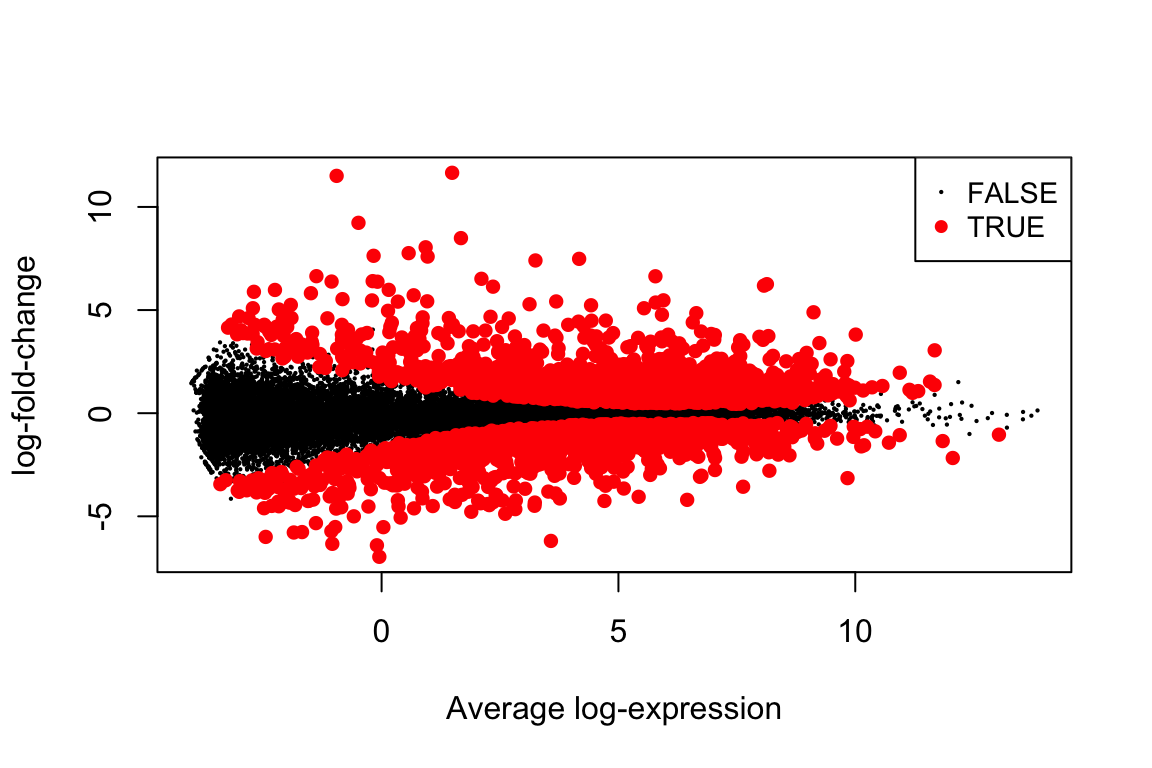
You might also consider using my topconfects package. This will find the largest confident effect sizes, while still correcting for multiple testing.
library(topconfects)
limma_confects(fit, "C1")
## $table
## rank index confect effect AveExpr name gene_name
## 1 12120 6.968 11.506653 -0.9495193 ENSG00000179593 ALOX15B
## 2 9499 5.925 7.404889 3.2480486 ENSG00000163884 KLF15
## 3 3272 5.896 11.655103 1.4890296 ENSG00000109906 ZBTB16
## 4 2230 5.410 6.255818 8.1342789 ENSG00000101347 SAMHD1
## 5 8175 5.408 7.483462 4.1705059 ENSG00000152583 SPARCL1
## 6 1836 5.267 6.637774 5.7809158 ENSG00000096060 FKBP5
## 7 9220 -5.047 -6.192439 3.5750054 ENSG00000162692 VCAM1
## 8 5156 4.567 8.488366 1.6752492 ENSG00000127954 STEAP4
## 9 10420 4.567 8.042925 0.9298793 ENSG00000168309 FAM107A
## 10 19752 4.567 9.229434 -0.4883206 ENSG00000250978 RP11-357D18.1
## gene_biotype mean_lcpm dispersion_before dispersion_trend
## protein_coding -0.9495193 0.142315693 0.32508630
## protein_coding 3.2480486 0.026366143 0.03478772
## protein_coding 1.4890296 1.213772655 0.08708543
## protein_coding 8.1342789 0.003891762 0.01721555
## protein_coding 4.1705059 0.158849347 0.02419826
## protein_coding 5.7809158 0.062948554 0.01694075
## protein_coding 3.5750054 0.017149286 0.03020135
## protein_coding 1.6752492 0.671533889 0.07840854
## protein_coding 0.9298793 0.447274209 0.11969603
## processed_transcript -0.4883206 0.759195732 0.25977988
## dispersion_after
## 0.4377782
## 0.7579151
## 13.9377231
## 0.2260608
## 6.5644939
## 3.7158076
## 0.5678317
## 8.5645506
## 3.7367506
## 2.9224578
## ...
## 5227 of 23171 non-zero log2 fold change at FDR 0.05
## Prior df 7.1