This vignette demonstrates the vst function for Variance
Stabilizing Transformation (VST) of count data, as well as various
useful diagnostic plots.
Variance Stabilizing Transformation
Filtering is recommended as a first step before using
vst. Use your favourite filtering method, for example
edgeR::filterByExpr provides a slightly better approach
than what I do here:
keep <- rowSums(counts >= 10) >= 4
table(keep)
#> keep
#> FALSE  TRUE
#> 47538 16139

counts_kept <- counts[keep,,drop=FALSE]
We can now apply a VST using vst. By default Anscombe’s
VST for negative binomial data is used. This is like a log2
transformation for large counts, but is a bit different for small
counts. The data is also normalized for library size, by default with
TMM adjustment. Here I request values that can be interpreted as log2
CPM.
lcpm <- vst(counts_kept, cpm=TRUE)
#> Dispersion estimated as 0.01570271
A better estimate of the dispersion can be obtained by specifying a design matrix. This ensures real signal in the data is not treated as noise.
design <- model.matrix(~ 0 + dex + cell, data=colData(airway))

lcpm <- vst(counts_kept, design=design, cpm=TRUE)
#> Dispersion estimated as 0.008576137
Stability plot
plot_stability allows assessment of how well the
variance has been stabilized. Ideally this will produce a horizontal
line, but counts below 5 will always show a drop off in variance.
plot_stability(lcpm, counts_kept, design=design)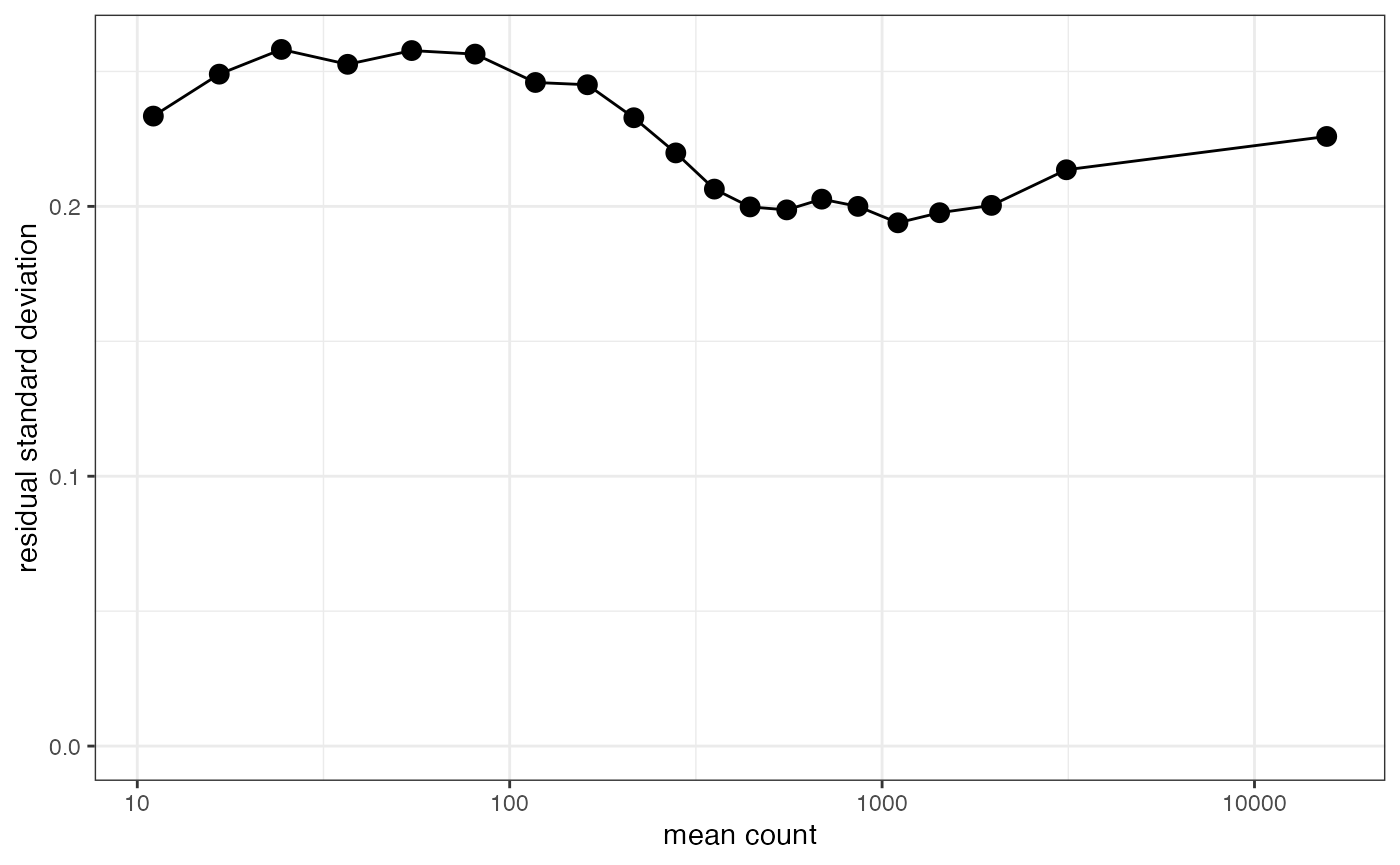
Biplot
plot_biplot provides a two-dimensional overview of your
samples and genes using Principle Components Analysis (similar concept
to plotMDS in limma).
plot_biplot(lcpm)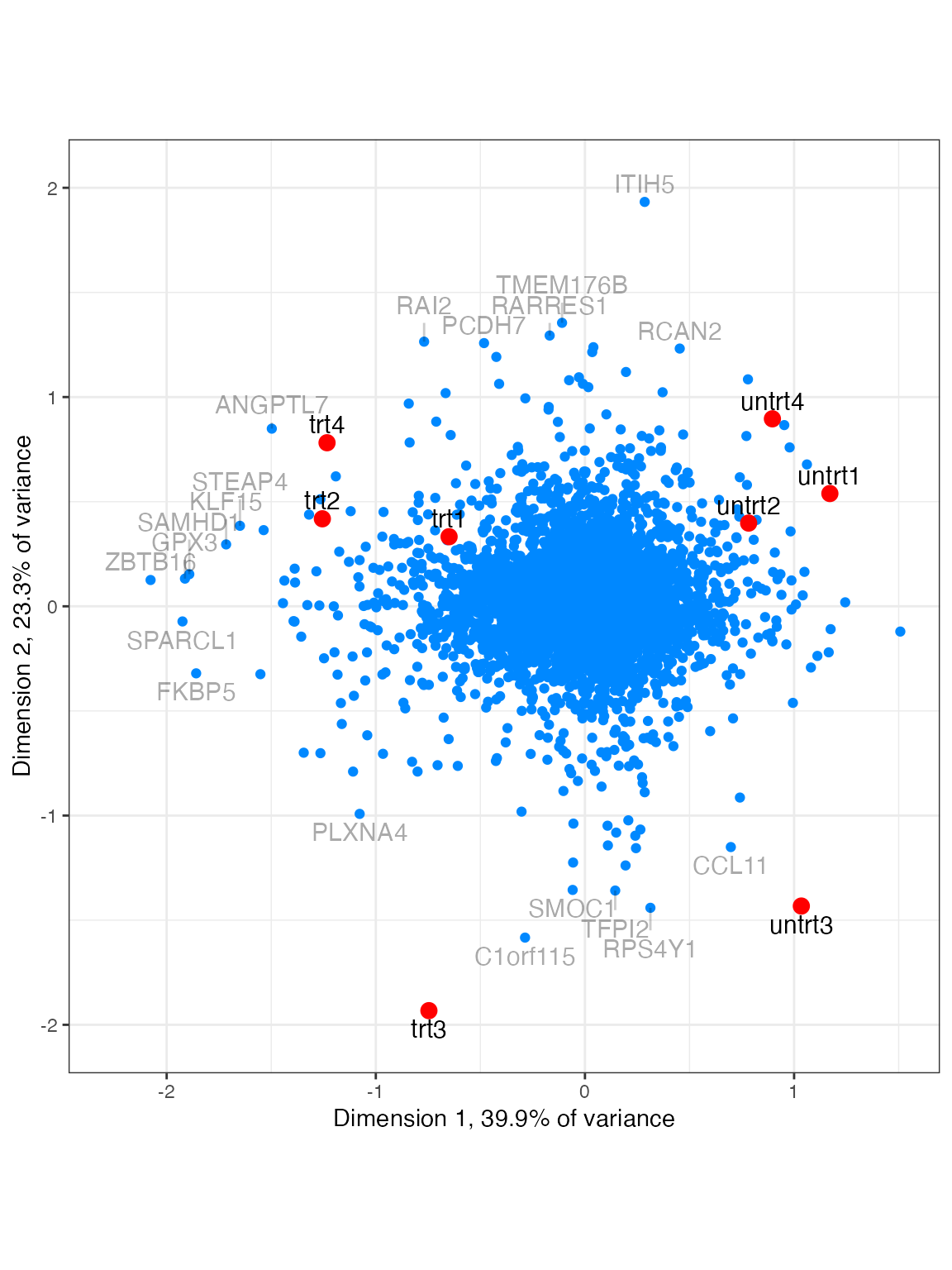
Heatmap
plot_heatmap draws a heatmap. Specify n=...
to only show the top genes by span of values.
plot_heatmap(lcpm, n=50)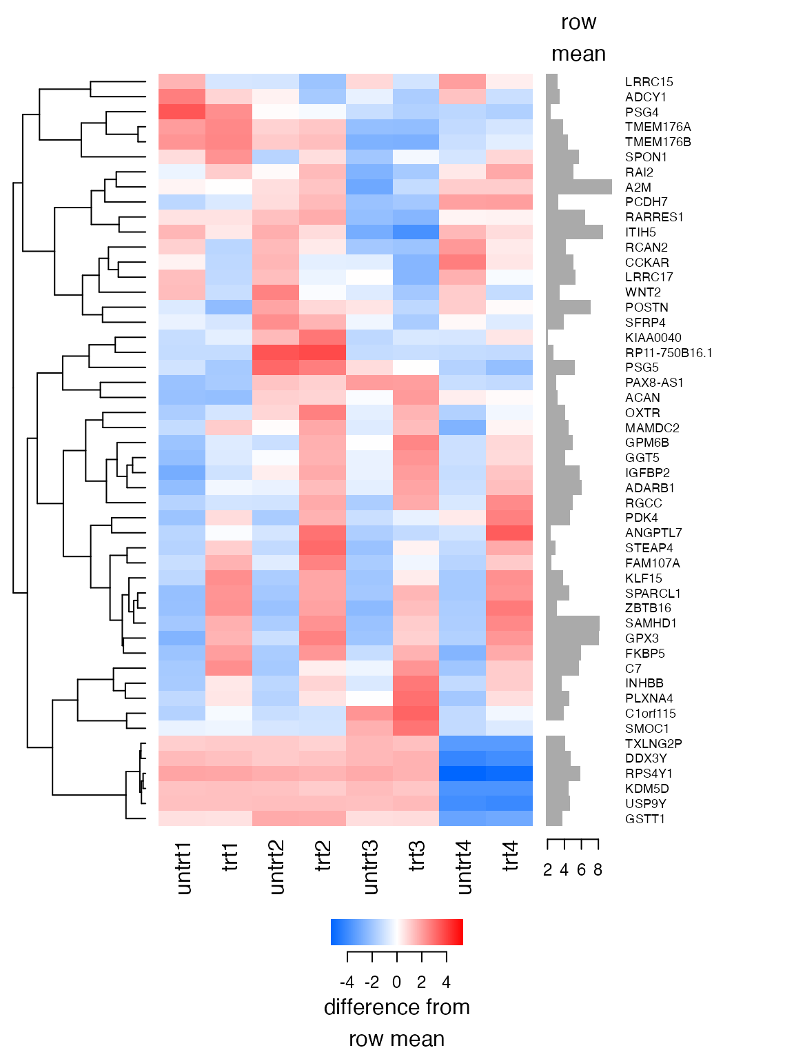
Shiny report
Varistran’s various diagnostic plots are also available as a Shiny app, which can be launched with:
shiny_report(lcpm, counts_kept)