This article puts samesum_log2_norm() and
samesum_log2_cpm() through their paces.
Example usage
lnorm <- samesum_log2_norm(counts)

colSums(lnorm)
#>   untrt1     trt1   untrt2     trt2   untrt3     trt3   untrt4     trt4
#> 123445.8 123445.8 123445.8 123445.8 123445.8 123445.8 123445.8 123445.8
attr(lnorm,"sum")
#> [1] 123445.8
attr(lnorm,"samples")
#>     name    scale true_lib_size adjusted_lib_size
#> 1 untrt1 2.006479      20637971          21667160
#> 2   trt1 1.760615      18809481          19012176
#> 3 untrt2 2.424240      25348649          26178399
#> 4   trt2 1.293811      15163415          13971346
#> 5 untrt3 2.342422      24448408          25294871
#> 6   trt3 2.778465      30818215          30003524
#> 7 untrt4 1.861340      19126151          20099863
#> 8   trt4 1.833587      21164133          19800165
plot_heatmap(
  lnorm,
  feature_labels=rowData(airway)$symbol,
  n=50, baseline_to=0)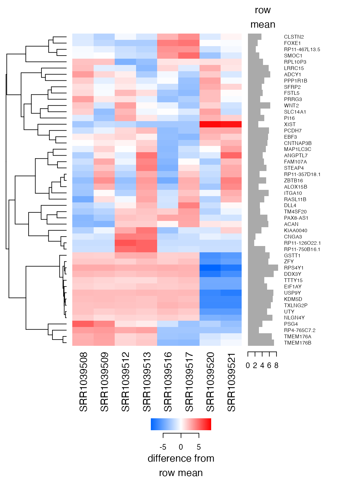
plot_biplot(lnorm, feature_labels=rowData(airway)$symbol)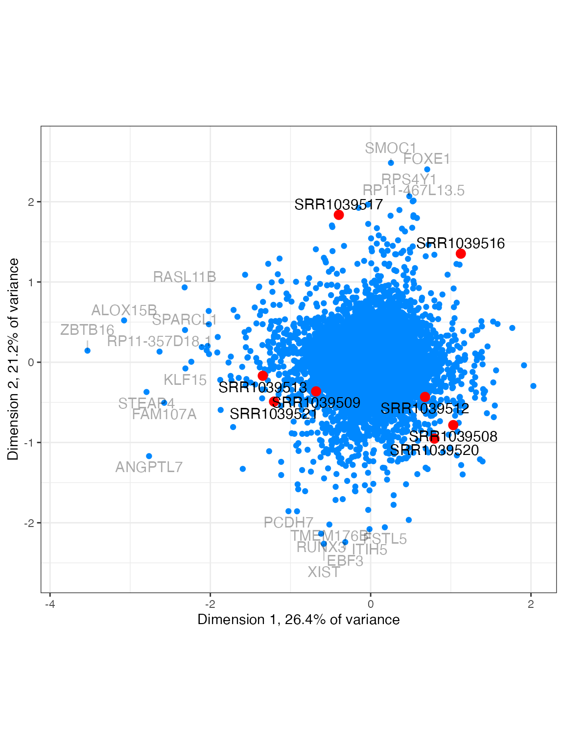
Filtering
Some analysis methods don’t work well with features that are nearly all zero. In particular we suggest filtering before using limma. However samesum transformation works fine with very sparse data, so we suggest transforming your data before filtering it. This allows filtering to be applied fairly across samples with different scale values.
Here the data has four replicates per treatment group, so for each
gene I require some level of expression in at least four samples. This
is similar to the strategy used by edgeR::filterByExpr.
keep <- rowSums(lnorm >= 2.5) >= 4
table(keep)
#> keep
#> FALSE  TRUE
#> 47530 16147
lnorm_filtered <- lnorm[keep,]

design <- model.matrix(~ 0 + dex + cell, data=colData(airway))
plot_stability(lnorm_filtered, counts[keep,], design=design)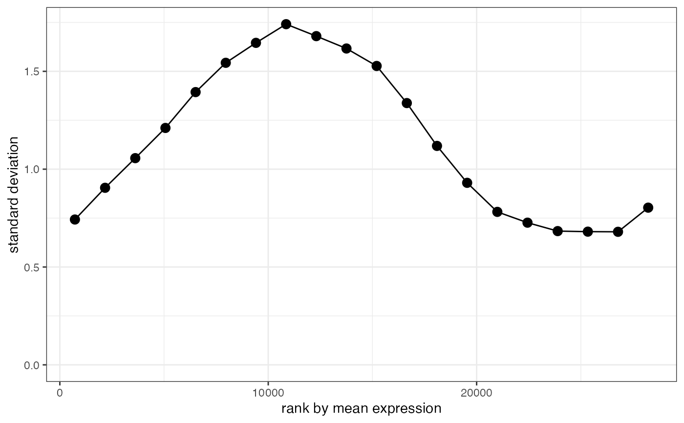
You can provide a larger target scale for greater variance stabilization
The default target scale parameter is 2, which may produce noisy results for features with low abundance. This scale parameter can be increased.
lnorm_10 <- samesum_log2_norm(counts, scale=50)

colSums(lnorm_10)
#>   untrt1     trt1   untrt2     trt2   untrt3     trt3   untrt4     trt4
#> 48190.48 48190.48 48190.48 48190.48 48190.48 48190.48 48190.48 48190.48
attr(lnorm_10, "samples")
#>     name    scale true_lib_size adjusted_lib_size
#> 1 untrt1 50.13240      20637971          21644530
#> 2   trt1 44.35235      18809481          19149007
#> 3 untrt2 58.64445      25348649          25319585
#> 4   trt2 33.46828      15163415          14449840
#> 5 untrt3 57.53114      24448408          24838916
#> 6   trt3 69.50408      30818215          30008201
#> 7 untrt4 45.59064      19126151          19683636
#> 8   trt4 47.37619      21164133          20454544

keep_10 <- rowSums(lnorm_10 >= 0.25) >= 4
table(keep_10)
#> keep_10
#> FALSE  TRUE
#> 47552 16125
lnorm_10_filtered <- lnorm_10[keep_10,]

plot_stability(lnorm_10_filtered, counts[keep_10,], design=design)
You can provide the target sum directly
By default, samesum_log2_norm chooses the target sum
based on the average sum from a first pass transformation of the data
with the target scale. You might instead provide this target sum
directly.
lnorm_sum <- samesum_log2_norm(counts, sum=1e5)

colSums(lnorm_sum)
#> untrt1   trt1 untrt2   trt2 untrt3   trt3 untrt4   trt4
#>  1e+05  1e+05  1e+05  1e+05  1e+05  1e+05  1e+05  1e+05
attr(lnorm_sum, "samples")
#>     name    scale true_lib_size adjusted_lib_size
#> 1 untrt1 4.711026      20637971          21695573
#> 2   trt1 4.132692      18809481          19032182
#> 3 untrt2 5.624991      25348649          25904631
#> 4   trt2 3.077556      15163415          14172993
#> 5 untrt3 5.449664      24448408          25097201
#> 6   trt3 6.483651      30818215          29858998
#> 7 untrt4 4.344943      19126151          20009660
#> 8   trt4 4.346977      21164133          20019024
For example you might want to ensure the chosen scale for each sample
is greater than some minimum. You could compute the first pass sums
yourself with colSums(log1p(counts/target_scale))/log(2)
and provide the minimum value as the target sum.
I propose to call the units of the target sum “dublins”, being roughly how many doublings of abundance are observed in each sample. You can think of this as the resolution at which we are looking at the data. Now we generally want the scale to be greater than, say, 0.5, and this will mean different technologies and sequencing depths will support different amounts of dublins.
If comparing multiple datasets, using a consistent target sum allows for consistent comparisons. For example the sum of squared log fold changes minus the sum of squared standard errors can be used as an unbiassed estimate of how much differential expression there is between two conditions. To render this consistent across multiple disparate datasets, a consistent number of dublins could be used.
You can also produce log2 CPM values
Counts Per Million (CPM) is a widely used unit for RNA-Seq data, so I
also provide a function to produce results in log2 CPM units. This is
quite similar to edgeR’s cpm function with
log=TRUE.
lcpm <- samesum_log2_cpm(counts)Zeros will no longer be zero. This is fine, log transformation is meant to transform positive values to cover the whole real line. It is convenient sometimes to pick a log transformation with a pseudocount that transforms zeros to zero, but it is not necessary.
You can check the value that zeros are transformed to.
min(lcpm)
#> [1] -3.434502
attr(lcpm, "zero")
#> [1] -3.434502

mean(colSums(2^lcpm-2^attr(lcpm,"zero")))
#> [1] 1e+06
Adjust your filtering appropriately.
Low library size samples produce a warning
Here I have downsampled the first sample to 1% of the original. The function gives a warning.
set.seed(563)
counts_sub <- counts
counts_sub[,1] <- rbinom(nrow(counts_sub), counts_sub[,1], 0.01)

lnorm_sub <- samesum_log2_norm(counts_sub)
#> Warning in samesum_log2_norm(counts_sub): 1 samples have been given a scale
#> less than 0.5. These may subsequently appear to be outliers as an artifact of
#> the transformation. Consider using a larger target scale or excluding these
#> samples from analysis.
You can examine the samples attribute for more details.
attr(lnorm_sub,"samples")
#>     name     scale true_lib_size adjusted_lib_size
#> 1 untrt1 0.0103538        205717          83191.73
#> 2   trt1 2.7133387      18809481       21801392.68
#> 3 untrt2 3.7132470      25348649       29835551.65
#> 4   trt2 2.0091857      15163415       16143596.90
#> 5 untrt3 3.5924834      24448408       28865228.65
#> 6   trt3 4.2665191      30818215       34281035.59
#> 7 untrt4 2.8609935      19126151       22987783.61
#> 8   trt4 2.8410567      21164133       22827594.11
Sample 1 is indeed an outlier now, and this is purely an artifact of the transformation:
plot_heatmap(lnorm_sub, feature_labels=rowData(airway)$symbol, n=50, baseline_to=0)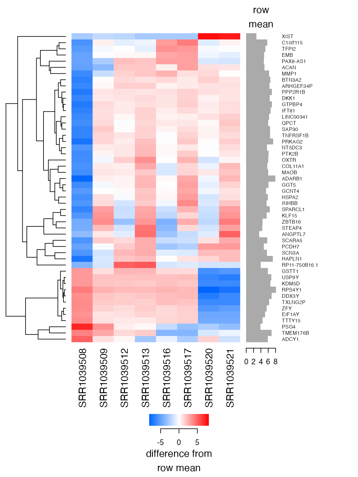
Increasing the scale parameter removes the warning and
fixes the problem. The cost is that we squash variability in genes with
low expression levels. It’s like we’ve reduced the “resolution” of the
data.
lnorm_sub_200 <- samesum_log2_norm(counts_sub, scale=200)

attr(lnorm_sub,"sum")
#> [1] 111245.9
attr(lnorm_sub_200,"sum")
#> [1] 23743.31
We’re now looking at the data at a resolution of 23,743 dublins, where previously we were looking at a resolution of 111,246 dublins.
plot_heatmap(lnorm_sub_200, feature_labels=rowData(airway)$symbol, n=50, baseline_to=0)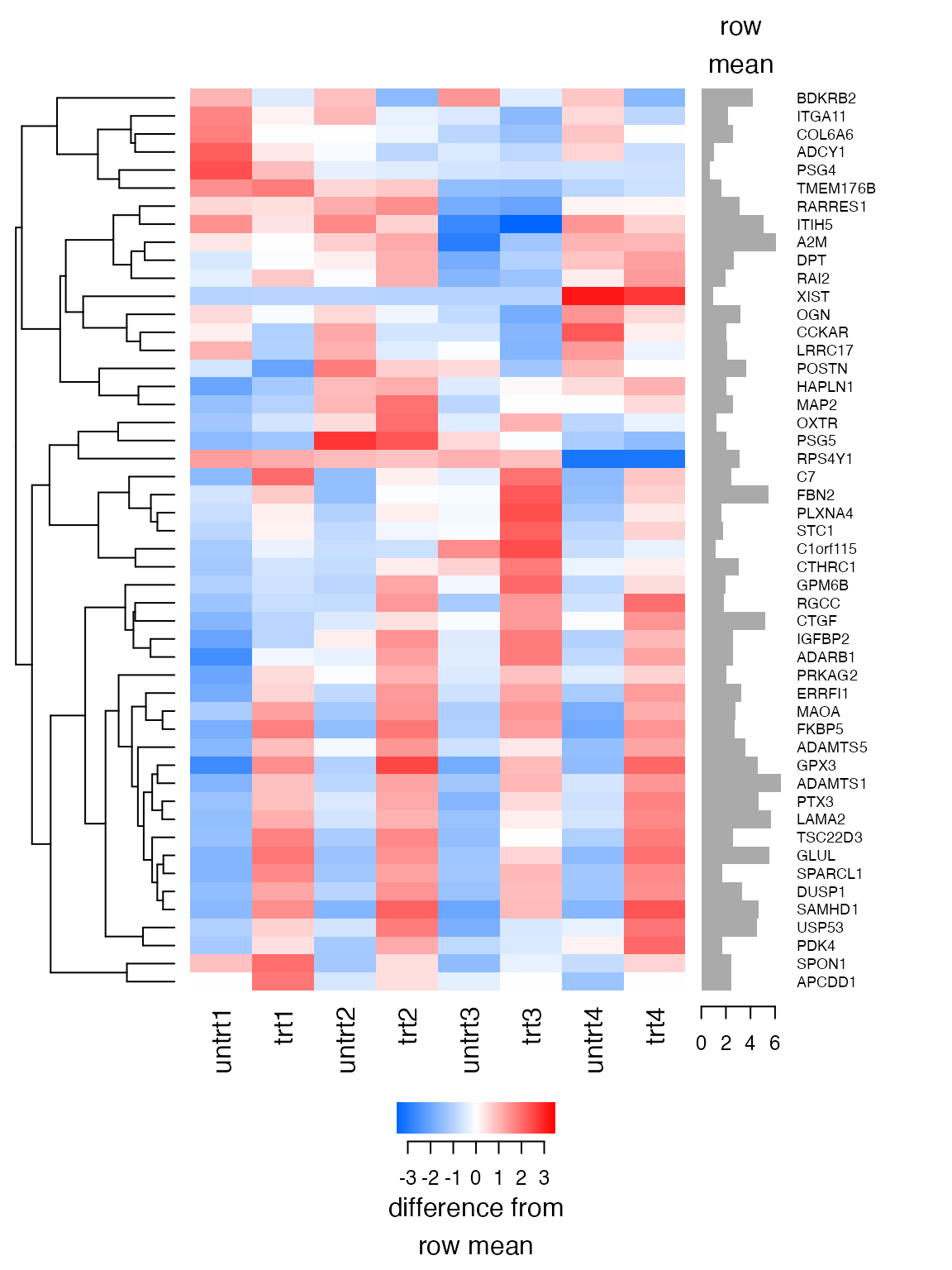
You will also get a warning if a sample is all zero.
counts_zeroed <- counts
counts_zeroed[,1] <- 0
lnorm_zeroed <- samesum_log2_norm(counts_zeroed)
#> Warning in samesum_log2_norm(counts_zeroed): 1 samples are entirely zero.
Or sometimes a sample has very low library size or complexity, and the scale underflows to zero.
counts_low <- counts_zeroed
counts_low[1,1] <- 1
lnorm_low <- samesum_log2_norm(counts_low)
#> Warning in samesum_log2_norm(counts_low): 1 samples where the scale has
#> underflowed and been given a value of zero. Please remove these samples.
Sparse matrices can be used
samesum_log2_norm transforms zeros to zeros, so the
matrix remains sparse. This can be useful for example with scRNA-Seq
data.
counts_sparse <- Matrix( assay(airway, "counts") )
lnorm_sparse <- samesum_log2_norm(counts_sparse)
class(lnorm_sparse)
#> [1] "dgCMatrix"
#> attr(,"package")
#> [1] "Matrix"