I will use the airway dataset from Bioconductor. In this data, the rows are genes, and columns are measurements of the amount of RNA in different biological samples. The data examines the effect of dexamethasone treatment on four different airway muscle cell lines.
Data normalization and filtering
I start with the usual mucking around for an RNA-Seq dataset to normalize and log transform the data, and get friendly gene names.
I also filter out genes with low variability (this also eliminates genes with low expression). This is mostly to keep the number of points manageable in langevitour.
library(langevitour)
library(airway)               # airway dataset
library(edgeR)                # RPM calculation
library(limma)                # makeContrasts
library(MASS)                 # ginv generalized matrix inverse
library(org.Hs.eg.db)         # Gene information
library(crosstalk)            # Communication with other htmlwidgets
library(DT)                   # Table htmlwidget
library(ggplot2)
library(dplyr)
library(tibble)

data(airway)

treatment <- colData(airway)$dex == "trt"
cell <- factor(c(1,1,2,2,3,3,4,4))
design <- model.matrix(~ 0 + cell + treatment)

dge <- airway |>
    assay("counts") |>
    DGEList() |>
    calcNormFactors()

# Convert to log2 Reads Per Million.
# prior.count=5 applies some moderation for counts near zero.
rpms <- cpm(dge, log=TRUE, prior.count=5)

# Only show variable genes (mostly for speed)
keep <- apply(rpms,1,sd) >= 0.25
table(keep)
#> keep
#> FALSE  TRUE
#> 48707 14970
y <- rpms[keep,,drop=F]

# Use shorter sample names
colnames(y) <- paste0(ifelse(treatment,"T","U"), cell)

# Get gene symbols and descriptions
genes <-
    left_join(
        tibble(ENSEMBL=rownames(y)),
        AnnotationDbi::select(
            org.Hs.eg.db,
            keys=rownames(y),
            keytype="ENSEMBL",
            columns=c("SYMBOL","GENENAME")),
        by="ENSEMBL") |>
    mutate(SYMBOL=ifelse(is.na(SYMBOL),ENSEMBL,SYMBOL)) |>
    group_by(ENSEMBL) |>
    summarize(SYMBOL=paste(SYMBOL,collapse="/"), GENENAME=paste(GENENAME,collapse="/"))

stopifnot(identical(genes$ENSEMBL, rownames(y)))
genes$AveExpr <- rowMeans(y) |> round(1)

# Colors for the samples
colors <- ifelse(treatment,"#f00","#080")
These are the first few rows of our normalized and log transformed data.
U = Untreated, T = Treated, 1 2 3 4 = cell line.
y[1:5,]
#>                   U1   T1    U2   T2   U3   T3   U4   T4
#> ENSG00000000003 4.97 4.55 5.140 4.84 5.51 5.14 5.30 4.83
#> ENSG00000000460 1.58 1.62 0.874 1.41 1.74 1.22 2.03 1.67
#> ENSG00000000971 7.22 7.57 7.955 8.21 8.07 8.52 8.04 8.62
#> ENSG00000001084 4.59 4.31 4.591 5.11 5.04 4.59 5.15 5.13
#> ENSG00000001167 4.20 3.63 4.236 3.63 4.73 4.30 4.21 3.75
Contrasts of interest
I now work out how to estimate a linear model and calculate contrasts of interest. The contrasts will be made available as extra axes in the langevitour plot.
coefficient_estimator <- MASS::ginv(design)

contrasts <- makeContrasts(
        average=(cell1+cell2+cell3+cell4)/4+treatmentTRUE/2,
        treatment=treatmentTRUE,
        "cell1 vs others" = cell1-(cell2+cell3+cell4)/3,
        "cell2 vs others" = cell2-(cell1+cell3+cell4)/3,
        "cell3 vs others" = cell3-(cell1+cell2+cell4)/3,
        "cell4 vs others" = cell4-(cell1+cell2+cell3)/3,
        levels=design)

contrastAxes <- t(coefficient_estimator) %*% contrasts

contrastAxes
#>       Contrasts
#>        average treatment cell1 vs others cell2 vs others cell3 vs others
#>   [1,]   0.125     -0.25           0.500          -0.167          -0.167
#>   [2,]   0.125      0.25           0.500          -0.167          -0.167
#>   [3,]   0.125     -0.25          -0.167           0.500          -0.167
#>   [4,]   0.125      0.25          -0.167           0.500          -0.167
#>   [5,]   0.125     -0.25          -0.167          -0.167           0.500
#>   [6,]   0.125      0.25          -0.167          -0.167           0.500
#>   [7,]   0.125     -0.25          -0.167          -0.167          -0.167
#>   [8,]   0.125      0.25          -0.167          -0.167          -0.167
#>       Contrasts
#>        cell4 vs others
#>   [1,]          -0.167
#>   [2,]          -0.167
#>   [3,]          -0.167
#>   [4,]          -0.167
#>   [5,]          -0.167
#>   [6,]          -0.167
#>   [7,]           0.500
#>   [8,]           0.500
Principal Components
I will also supply Principal Components as extra axes in the plot. When doing the PCA, I don’t use scaling because the data is already all in comparable units of measurement (log2 RPM). From the scree plot, four components seems reasonable. I then apply varimax rotation of these axes to make them more easily interpretable.
pca <- prcomp(t(y), center=TRUE, scale=FALSE, rank=4)
vmAxes <- pca$x %*% varimax(pca$rotation, normalize=FALSE)$rotmat
colnames(vmAxes) <- paste0("VM",seq_len(ncol(vmAxes)))

plot(pca)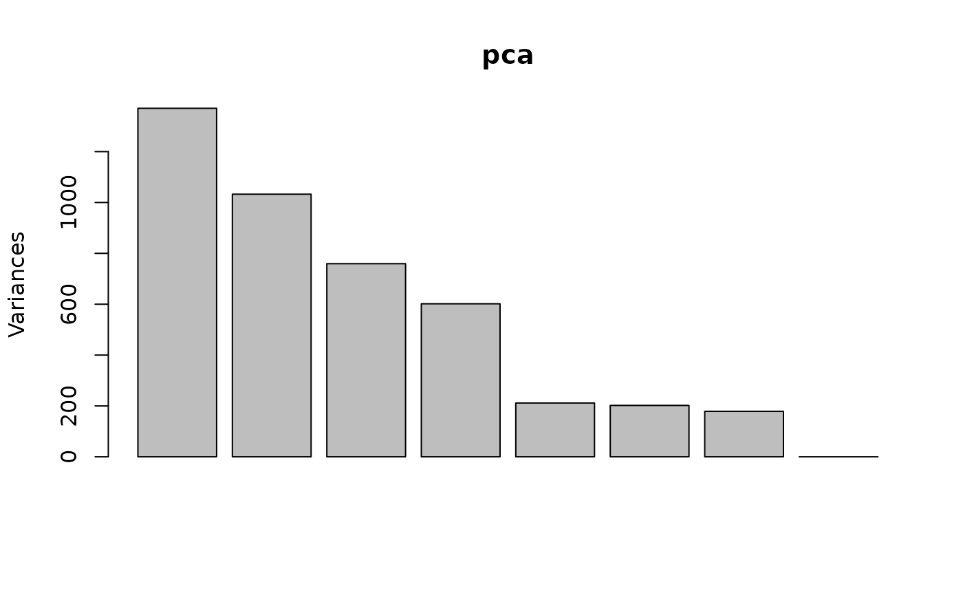
Plot the data with langevitour
We are now ready to do the langevitour plot.
A key tool we will use is deactivating an axis by unchecking its checkbox. Langevitour will then only show projections of the data that are orthogonal to the deactivated axis.
Things to try:
Your first step will be to , since this is large and uninformative.
Try dragging different axes onto the plot.
Try setting the guide to . You may also need to increase the strength of the guide. This will look for projections in which some genes have large differential expression.
Drag treatment onto the plot, and deactivate the “average” axis and each of the “cell vs others” axes. Also ensure point repulsion is “none”. The remaining variation orthogonal to the treatment axis should be purely random variation. You can compare this to the variation along the treatment axis. This is a visual version of a statistical test called a “rotation test”. For each gene, we can compare its projection along the treatment axis to the random projections being shown orthogonal to the treatment axis. If it is extreme compared to these random projections we reject that treatment had no effect on the gene. ((There is a bit more that needs to be said here, about multiple testing.)) ()
shared <- SharedData$new(genes)

langevitour(
    y, name=genes$SYMBOL, scale=15, center=rep(3,8),
    extraAxes=cbind(contrastAxes, vmAxes),
    axisColors=colors, link=shared, elementId="myWidget")
datatable(shared, rownames=FALSE) # Linked table widgetNotes:
- The main interest is a small number of genes affected by the treatment.
- We can also see small numbers of genes expressing differently in the different cell-lines.